Category: MiWORD of the Day

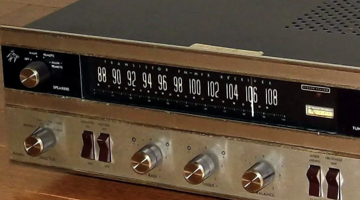
At first glance, radiomics sounds like the name of a futuristic radio station:
“Welcome back to Radiomics FM, where all your favorite tumors are top hits!”

But no, radiomics isn’t about DJs, airwaves, or tuning into late-night medical jams. Instead, it’s about something even cooler: finding hidden patterns buried deep inside medical images and letting ML models “listen” to what those patterns are trying to say.

Imagine staring at a blurry shadow on the wall. Is it a cat? A chair? A really bad haircut?

Medical images, like CT scans, MRIs, and ultrasounds, can feel just as mysterious to the naked eye. They’re full of shapes, textures, and intensity patterns that look like a mess… until you start digging deeper.

That’s where radiomics comes in. Radiomics acts like a detective with a magnifying glass, picking out tiny, subtle clues inside the fuzziness. It systematically extracts hundreds, sometimes even thousands, of quantitative features from images, including:

• Texture features (like entropy, smoothness, or roughness)
• Shape descriptors (capturing the size, compactness, or irregularity of objects)
• First-order intensity statistics (how bright or dark different regions are)
• Higher-order patterns (relationships between pixel groups, like GLCM and GLRLM matrices)
  

Each of these features gets transformed into structured data, powerful numbers that machine learning models can analyze to predict clinical outcomes. Instead of relying only on human interpretation, radiomics opens a new window into understanding:

• Will the tumor grow fast or stay slow?
• Will the patient respond well to a certain treatment?
• Could we detect early signs of disease long before symptoms appear?

Fun Fact: Radiomics can spot differences so subtle that even expert radiologists can’t always detect them. It’s like giving X-ray vision… to an already X-rayed image. By turning complex images into rich datasets, radiomics is revolutionizing how we approach personalized medicine. It allows researchers to build predictive models, identify biomarkers, and move toward earlier, more accurate diagnoses without the need for additional invasive biopsies or surgeries.

Radiomics reminds us that in science, and in life, what we see isn’t always the full truth. Sometimes, it’s the quiet, hidden patterns that matter most. So next time you see a grayscale ultrasound or a mysterious CT scan, remember: Behind those shadows, there’s a secret world of patterns and numbers just waiting to be uncovered.

Now, try using radiomics in a sentence by the end of the day!

Serious: “Radiomics enables earlier detection of subtle tumor changes that are invisible to the human eye.”

Not so serious: “I’m using radiomics to decode my friend’s emotions, because reading faces is harder than reading scans.”

See you next time in the blogosphere, and don’t forget to tune out Radiomics FM!

Phoebe (Shih-Hsin) Chuang

OK, what comes to mind when you hear the word diffusion? Perfume spreading through a room? A drop of ink swirling into a glass of water? When I first heard the terms “diffusion model”, I thought of my humidifier, chaotically diffusing water droplets in my room.

But today, diffusion has taken on a very new meaning in the world of medical imaging!

You’ve probably heard a lot about GPT recently, models that can generate almost anything: stories, poems, even computer code. But did you know that alongside GPT for text, there are other types of models that generate images, like beautiful paintings, photorealistic pictures… and yes, even medical images?

This is where the “diffusion” in diffusion models comes in! Just like my humidifier slowly releases tiny water droplets into the air, diffusion models spread random noise across an image and then cleverly gather it back together to form something meaningful! In my case, instead of a cat jumping because they saw a cucumber, I generate gastrointestinal tract images from their segmentation masks! (Yes, I agree with you, I am cooler)

But what are segmentation masks?

Elementary, my dear Watson! Segmentation masks are like a topological map, showing the exact locations that Sherlock Holmes (in this case, the radiologist) would search for hidden clues, such as tumors, organs, vessels, to uncover cancerous Moriarty’s next plan. Super important when doctors need to know exactly where to operate or how a disease is spreading.

Until recently, generating these masks required lots of manual work from radiologists, or tons of carefully labeled data. But now?

By training diffusion models properly, we can synthesize realistic segmentation masks, even when data is limited. That means more diverse, more accurate, and more creative ways to augment medical datasets for training better AI models.

It’s like equipping our medical research toolbox with a team of colorful GPUs, each one working like a tireless laboratory assistant, swiftly and precisely creating endoscopy images at the click of a button, generating in moments what used to take hours of painstaking effort. This lets you breathe easy, knowing that your next endoscopy won’t need to be fed into an AI model, thus sparing patient privacy and giving medical professionals more time to focus on what truly matters!

Thank you for reading, and I’ll see you in the blogosphere!

Xin Lei Lin

Remember that famous Spider-Man meme where two Spider-Men are pointing at each other, yelling “You’re me!”? That’s basically the spirit of the McNemar Test. It’s a statistical tool that checks whether the same group of people changes their answers under two different conditions.

Think of it like this: yesterday everyone swore bubble tea was the best, but today half of them suddenly insist black coffee is the only way to survive finals. The McNemar Test is the referee here—it counts how many people actually flipped sides and asks, “Okay, is this change big enough to matter, or is it just random mood swings?”

The McNemar Test works on paired data. The total numbers don’t matter as much as the people who changed their minds.

People who said “yes” before and still say “yes” after → not interesting.

People who said “no” before and still say “no” after → also not interesting.

The stars of the show? Those who said “yes” before and “no” after, and those who said “no” before and “yes” after. The test compares these two groups. If the difference between them is large, it means the change is real, not just random noise.

In clinical research this is super important. Suppose a study tests whether a new drug actually helps with a disease. A total of 314 patients are observed both before and after treatment. Here’s the data:

Here’s what’s going on: 101 stayed sick before and after. 33 stayed healthy before and after.

121 improved (from sick → healthy). 59 worsened (from healthy → sick).

Now, McNemar steps in with this formula:

That comes out to 21.35, which is way too extreme to happen by chance (p < 0.001). Translation: the drug worked—the number of patients who got better is significantly higher than those who got worse.

In medicine (or in evaluating machine learning models), it’s not enough to just report an overall accuracy. What really matters is whether the changes—improvements or mistakes—are meaningful and consistent. The McNemar Test is a simple way to check if those differences are statistically real.

Now let’s use McNemar Test in a sentence.

Serious: In a clinical trial, the McNemar Test showed that significantly more patients improved after treatment than worsened, proving the drug’s effectiveness.

Less Serious: Yesterday my friend swore pizza was the best food on earth. Today she switched to sushi. According to McNemar, this isn’t just random—it’s a statistically significant betrayal.

See you in the blogosphere!

Nathan Liu

Have you ever tried to take a perfect vacation photo in Toronto, only to find your friend’s face is a mysterious smudge and the CN Tower looks like it’s melting? Blur has a way of sneaking into our lives, and it is everywhere. Sometimes it is more fascinating than you might think.

The smudge you see in your photo is blur. Blur has existed since the first camera was invented because film or sensors need time to gather light. If either the subject or the camera moves during this exposure time, the image appears blurred. In our discussion, we will focus on motion blur caused by fast movement, rather than unrelated effects like pixelation or mosaic artifacts. You might have experienced motion blur when taking a shaky phone photo, wearing foggy glasses, or watching a baseball fly past at incredible speed. But blur is not always a flaw.

In the world of art, blur has often been a feature rather than a mistake. Think of Claude Monet’s Water Lilies (link, copyright by The MET — highly recommend seeing it in person and viewing it from different distances): soft edges, blended colors, shapes shimmering in the light. Or consider long-exposure photographs of city traffic, where headlights stretch into glowing ribbons. In these cases, blur captures motion, mood, and mystery, transforming the ordinary into something extraordinary. Even in classic cinema, motion blur helps create a sense of speed or dreamlike atmosphere. In sports, blur can tell an entire story. The fastest recorded baseball pitch reaches 105.8 miles per hour, far too fast for the human eye to follow clearly. To freeze it, cameras must shoot at over 1,000 frames per second. A racecar streaking past the finish line or a sprinter in motion may appear as streaks of color, yet our brains still understand exactly what is happening. Motion blur, in these cases, is not a mistake; it is evidence of speed and energy.

In science, blur can reveal a very different kind of truth. Consider echocardiography, an ultrasound imaging method for the heart. These moving pictures help doctors assess heart function, blood flow, and valve performance. Yet even the tiniest shake of the probe, a restless patient, or the natural motion of the heartbeat can smear crucial details. There is even a trade-off between frame rate and depth of view: a typical knee ultrasound operates at around 20 frames per second, while heart ultrasound often reaches about 50 frames per second. A blurry heart chamber is more than an inconvenience; it can obscure the clues doctors need to make the right decision. Other imaging fields, such as X-ray or MRI, face similar challenges with motion blur. Interestingly, scientists also study the patterns of blur to improve image quality, since sometimes the “smudge” itself contains useful information about movement or structure.

Blur can be playful, expressive, and at times essential. It reminds us that seeing clearly is not always straightforward and that what appears imperfect can still hold meaning. From the sweep of a painter’s brush to the rhythm of a beating heart on a screen, blur reflects a world that is always moving and changing. Sometimes, beauty and truth live within that very imperfection.

Now for the fun part — using blur in a sentence by the end of the day:
Serious: Did you notice the blur in the long-exposure shot of the city at night? The headlights look like flowing rivers of light.
Less serious: While running to catch the bus, I accidentally created a blur of people in my phone photo. What a perfect accidental art piece.

…I’ll see you in the blogosphere.

Qifan Yang

Look! You’ve finally made it to Canada! You gloriously take in the view of Lake Ontario when your friend beside you exclaims, “Look, they have beaver tails!” You excitedly scan the lake, asking, “Where?” 

“There!”

“Where?”

“There!”

You see no movement from the lake. It isn’t until your friend pulls you to the front of a storefront says “BeaverTails” with a picture of delicious pastries that you realize they didn’t mean actual beavers’ tails. It turns out you were looking at the wrong place the whole time!

Often times, it’s easy for us to quickly identify objects because we know the context of where things should be. These are the kinds of things we take for granted, until it’s time to hand the same tasks over to machines. 

In medical imaging, experts label what are called Regions of Interests (ROIs), which are specific areas of a medical image that contain pathology, such as the specific area of a lesion. Having labelled ROIs are important, as it can help prevent extra time from being wasted on analyzing non-relevant areas of an image, especially since medical images contain complex structures that take time to interpret. But in the area of machine learning (ML) in medical imaging, having labelled ROIs is also useful because it can help with training ML models that classify whether a medical image contains a pathology or not; with ROIs identified, cropping can be done during the preprocessing of images so that only relevant areas of images are compared for the model to learn differences between positive and negative images faster.

In fact, having ROIs is so important, there is an entire field in artificial intelligence dedicated to it: Computer Vision. The field of computer vision focuses on automating the extraction of ROIs in images or videos, which plays a critical role in the mechanization of tasks like object detection and tracking for things like self-driving cars. In object detection, for example, things like ROI Pooling can be utilized; this is where multiple ROIs are used to obtain input feature maps, from which maximum values are used to detect the presence of features, giving rise to the ability to identify many objects at once – this is extremely useful, especially once you’re on the road and there are 10 other cars around you!

Now, the fun part: using Region of Interest in a sentence!

Serious: The coordinates of ROIs are given for the positive mammogram images in the dataset I’m using. Maybe I could use Grad-CAM to see if the ML breast cancer classification model I’m using uses the same regions of the image to arrive at its classification decision; this way, I can see if its decision making aligns with the decision making of radiologists.

Less serious: I forced my friend to watch my favorite movie with me, but I can’t lie – I think the attractive male lead was her only region of interest!

See you in the blogosphere,

Yan Qing Lee

According to the dictionary, the term “adversarial” refers to a situation where two parties or sides oppose each other. But what about the “adversarial example”? Does it imply an example of two opposing sides? In a way, yes.

In machine learning, an example is one instance of the dataset. Adversarial examples are examples with calculated and imperceptible perturbation that tricks the model into the wrong prediction but look the same to humans. So “adversarial”, in this case, indicates opposition between something (or human) and the model. The adversarial examples are intentionally crafted to trick the model by exploiting its vulnerabilities.

How it works? There are many ways to find weak spots and generate adversarial examples, but FGSM is one classic way, and the goal is to make small changes to a picture such that it outputs the wrong prediction. First, we input the model with the picture. Assume the model outputs the correct prediction, so the loss function, which represents the difference between the prediction and the true label, will be low. Second, we compute the gradient of the loss function to tell us whether we should add or subtract a certain value epsilon to each pixel to make the loss bigger. Epsilon is typically very small, resulting in a tiny change to the value. Now, we have a picture that looks the same as the original but will trick the model into the opposite prediction!

One exciting property of adversarial examples is their transferability. It is known that adversarial examples created for one model can also trick other unknown models. This might be due to inherent flaws in the pattern recognition mechanisms of all models and, sometimes, model similarities, allowing these adversarial examples to exploit common vulnerabilities and lead to incorrect predictions.

Now, use “adversarial example” in a sentence by the end of the day: 

Kinda Serious: “Oh I can’t believe my eyes. I am seeing a dog right here and the model says it’s a cupcake…So you’re saying it might be an adversarial image? What even is that? The model is just dumb.”

Less Serious: Apparently, the movie star has an adversarial relationship with the media, but which stars have a good relationship with the media nowadays?

See you in the blogosphere,

Yuxi Zhu

Imagine you’re trying to compare two images—not just any images, but complex medical images like MRIs or X-rays. You want to know how similar they are, but traditional methods like simply comparing pixel values don’t always capture the whole picture. This is where Learned Perceptual Image Patch Similarity, or LPIPS, comes into play.

Learned Perceptual Image Patch Similarity (LPIPS) is a cutting-edge metric for evaluating perceptual similarity between images. Unlike traditional methods like Structural Similarity Index (SSIM) or Peak Signal-to-Noise Ratio (PSNR), which rely on pixel-level analysis, LPIPS utilizes deep learning. It compares images by passing them through a pre-trained convolutional neural network (CNN) and analyzing the features extracted from various layers. This approach allows LPIPS to capture complex visual differences more closely aligned with human perception. It is especially useful in applications such as evaluating generative models, image restoration, and other tasks where perceptual accuracy is critical.

Why is this important? In medical imaging, where subtle differences can be crucial for diagnosis, LPIPS provides a more accurate assessment of image quality, especially when images have undergone various types of degradation, such as noise, blurring, or compression.

Now, let’s use LPIPS in sentences!

Serious: When evaluating the effectiveness of a new medical imaging technique, LPIPS was used to compare the generated images to the original scans, showing that it was more sensitive to perceptual differences than traditional metrics.

Less Serious: I used LPIPS to compare my childhood photos with recent ones. According to the metric, I’ve definitely “degraded” over time!

See you in the blogosphere!

Jingwen (Lisa) Zhong

Volumetric rendering stands at the forefront of visual simulation technology. It intricately models how light interacts with myriad tiny particles to produce stunningly realistic visual effects such as smoke, fog, fire, and other atmospheric phenomena. This technique diverges significantly from traditional rendering methods that predominantly utilize geometric shapes (such as polygons in 3D models). Instead, volumetric rendering approaches these phenomena as if they are composed of an immense number of particles. Each particle within this cloud-like structure has the capability to absorb, scatter, and emit light, contributing to the overall visual realism of the scene. 

This is not solely useful for generating lifelike visual effects in movies and video games; it also serves an essential function in various scientific domains. Volumetric rendering enables the visualization of intricate three-dimensional data crucial for applications such as medical imaging, where it helps in the detailed analysis of body scans, and in fluid dynamics simulations, where it assists in studying the behavior of gases and liquids in motion. This technology, thus, bridges the gap between digital imagery and realistic visual representation, enhancing both our understanding and our ability to depict complex phenomena in a more intuitive and visually engaging manner. 

How does this work? 

Let’s start by talking about direct volume rendering. Instead of trying to create a surface for every object, this technique directly translates data (like a 3D array of samples, representing our volumetric space) into images. Each point in the volume, or voxel , contains data that dictates how it should appear based on how it interacts with light. 

For example, when visualizing a CT scan, certain data points might represent bone, while others might signify soft tissue. By applying a transfer function—a kind of filter—different values are mapped to specific colors and opacities. This way, bones might be made to appear white and opaque, while softer tissues might be semi-transparent. 

The real trick lies in the sampling process. The renderer calculates how light accumulates along lines of sight through the volume, adding up the contributions of each voxel along the way. It’s a complex ballet of light and matter, with the final image emerging from the cumulative effect of thousands, if not millions, of tiny interactions. 

Let us make this a bit more concrete. We first have transfer functions, a transfer function maps raw data values to visual properties like color and opacity. Let us represent the color assigned to some voxel as C(v) and the opacity as α(v). For each pixel in the final image, a ray is cast through the data volume from the viewer’s perspective. For this we have a ray equation: 

Where P(t) is a point along the ray at parameter 𝑡, P₀ is the ray’s origin, and is the normalized direction vector of the ray. As the ray passes through the volume, the renderer calculates the accumulated color and opacity along the ray. This is often done using compositing, where the color and opacity from each sampled voxel are accumulated to form the final pixel color. 

You probably used Volumetric Rendering 

Volumetric rendering transforms CT and MRI scans into detailed 3D models, enabling doctors to examine the anatomy and functions of organs in a non-invasive manner. A specific application includes most of the modern CT viewers. Volumetric rendering is key in creating realistic simulations and environments. In most AR applications, it is used under the hood to overlay interactive, three-dimensional images on the user’s view of the real world, such as in educational tools that project anatomical models for medical students. 

Now for the fun part (see the rules here), using volume rendering  in a sentence by the end of the day: 

Serious: The breakthrough in volumetric rendering technology has enabled scientists to create highly detailed 3D models of the human brain. 

Less Serious: I tried to use volumetric rendering to visualize my Netflix binge-watching habits, but all I got was a 3D model of a couch with a never-ending stream of pizza and snacks orbiting around it. 

…I’ll see you in the blogosphere. 

You might be thinking, “KL Divergence? Sounds exotic. Is it something to do with the Malaysian capital (Kuala Lumpur) or a measurement (kiloliter)?” Nope, and nope again! It stands for Kullback-Leibler Divergence, a fancy name for a metric to compare two probability distributions.

But why not just compare their means? After all, who needs these hard-to-pronounce names? Kullback… What was it again? That’s a good point! Here’s the catch: two distributions can have the same mean but look completely
different. Imagine two Gaussian distributions, both centered at zero, but one is wide and flat, while the other is narrow and tall. Clearly, not similar!

So, maybe comparing the mean and variance would work? Excellent thinking! But what if the distributions aren’t both Gaussian? For example, a wide and flat Gaussian and a uniform distribution (totally flat) might look similar visually, but the uniform distribution is not parametrized by a mean or variance. So, what do we compare?

Enter KL Divergence!

KL Divergence returns a single number that tells us how similar two distributions are, regardless of their types. The smaller the number, the more similar the distributions. But how do we calculate it? Here’s the formula (don’t worry, you don’t have to memorize it!).

Notice, if the distribution q has probability mass where p doesn’t, the KL Divergence will be large. Good, that’s what we want! But, if q has little mass where p has a lot, the KL Divergence will be small. Wait, that’s not what we want! No, it’s not, but luckily KL Divergence is asymmetric! KL(q || p) returns a different value than KL(p || q), so
we can compute both! Why are they different? I’ll leave that up to you to figure out!

KL Divergence in Action

Now, the fun part: using KL Divergence in a sentence!

Serious: Professor, can we approximate one distribution with another by minimizing the KL Divergence between them? That’s a great question! You’ve just stumbled on the idea behind Variational Inference.

Less Serious: Ladies and gentlemen, the KL Divergence between London and Kuala Lumpur is large, and so our flight time today will be 7 hour and 30 minutes. Please remember to stow your hand luggage in the overhead bins above you, fold your tray tables, and fasten your seatbelts.

See you in the blogosphere,
Benedek Balla

Have you ever tried to assemble a Lego set and ended up with mysterious extra pieces? Or perhaps you have cleaned up after a big party and found some confetti hiding in the corners days later? Welcome to the world of “residuals”!

Residuals pop up everywhere. It’s an everyday term but it’s actually fancier than just referring to the leftovers of a meal; it’s also a term used in regression models to describe the difference between observed and predicted values, or in finance to talk about what’s left of an asset. However, nothing I mentioned compares to the role residuals played in machine learning and particularly training deep neural networks.

When you learn an approximation of a function from an input space to an output space using backpropagation, the weights are updated based on the learning rate and gradients that are calculated through chain rule. As a neural network gets deeper, you have to multiply a small value—usually much smaller than 1—multiple times to pass it to the earliest layers, making the neural network excessively hard to optimize. This phenomenon prevalent in deep learning is call the vanishing gradient problem.

However, notice how deep layers of a neural network are usually composed by mappings that are close to identity. This is exactly why residual connections do their magic! Suppose your true mapping from input to output is h(x), and let the forward pass be f(x)+x. It follows that the mapping subject to learning would be h(x)-x, which is close to a zero function. This means f(x) would be way easier to learn under the vanishing gradient problem, since functions that are close to zero functions demand a lower level of sensitivity to each parameter, unlike the identity function.

Now before we dive too deep into the wizardry of residuals, should we use residual in a sentence?

Serious: Neuroscientists wanted to explore if CNNs perform similarly to the human brain in visual tasks, and to this end, they simulated the grasp planning using a computational model called the generative residual convolutional neural network.

Less serious: Mom: “What happened?”
Me: “Sorry Mom, but after my attempt to bake chocolate cookies, the residuals were a smoke-filled kitchen and a cookie-shaped piece of charcoal that even the dog wouldn’t eat”

See you in the blogosphere,
Mason Hu