MiWord of the Day Is… Fourier Transform!

Ok, a what Transform now??

In the early 1800s, Jean-Baptiste Joseph Fourier, a French mathematician and physicist, introduced the transform in his study of heat transfer. The idea seemed preposterous to many mathematicians at the time, but it has now become an important cornerstone in mathematics.

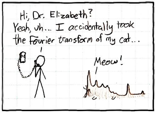
So, what exactly is the Fourier Transform? The Fourier Transform is a mathematical transform that decomposes a function into its sine and cosine components. It decomposes a function depending on space or time into a function depending on spatial or temporal frequency.

Before diving into the mathematical intricacies of the Fourier Transform, it is important to understand the intuition and the key idea behind it. The main idea of the Fourier Transform can be explained simply using the metaphor of creating a milkshake.

Imagine you have a milkshake. It is hard to look at a milkshake and understand it directly; answering questions such as “What gives this shake its nutty flavour?” or “What is the sugar content of this shake?” are harder to answer when we are simply given the milkshake. Instead, it is easier to answer these questions by understanding the recipe and the individual ingredients that make up the shake. So, how exactly does the Fourier Transform fit in here? Given a milkshake, the Fourier Transform allows us to find its recipe to determine how it was created; it is able to present the individual ingredients and the proportions at which they were combined to make the shake. This brings up the questions of how does the Fourier transform determine the milkshake “recipe” and why would we even use this transform to get the “recipe”? To answer the former question, we are able to determine the recipe of the milkshake by running it through filters that then extract each individual ingredient that makes up the shake. The reason we use the Fourier Transform to get the “recipe” is that recipes of milkshakes are much easier to analyze, compare, and modify than working with the actual milkshake itself. We can create new milkshakes by analyzing and modifying the recipe of an existing milkshake. Finally, after deconstructing the milkshake into its recipe and ingredients and analyzing them, we can simply blend the ingredients back to get the milkshake.

Extending this metaphor to signals, the Fourier Transform essentially takes a signal and finds the recipe that made it. It provides a specific viewpoint: “What if any signal could be represented as the sum of simple sine waves?”.

By providing a method to decompose a function into its sine and cosine components, we can analyze the function more easily and create modifications as needed for the task at hand.

 A common application of the Fourier Transform is in sound editing. If sound waves can be separated into their “ingredients” (i.e., the base and treble frequencies), we can modify this sound depending on our requirements. We can boost the frequencies we care about while hiding the frequencies that cause disturbances in the original sound. Similarly, there are many other applications of the Fourier Transform such as image compression, communication, and image restoration.

This is incredible! An idea that the mathematics community was skeptical of, now has applications to a variety of real-world applications.

Now, for the fun part, using Fourier Transform in a sentence by the end of the day:

Example 1:

Koby: “This 1000 puzzle is insanely difficult. How are we ever going to end up with the final puzzle picture?”

Eng: “Don’t worry! We can think of the puzzle pieces as being created by taking the ‘Fourier transform’ of the puzzle picture. All we have to do now is take the ‘inverse Fourier Transform’ and then we should be done!”

Koby: “Now when you put it that way…. Let’s do it!”

Example 2: 

Grace: “Hey Rohan! What’s the difference between a first-year and fourth-year computer science student?

Rohan: “… what?”

Grace: “A Fouri-y-e-a-r Transform”

Rohan: “…. (╯°□°)╯︵ ┻━┻ ”

I’ll see you in the blogosphere…

Parinita Edke

The MiDATA Word of the Day is…”clyster”

Holy mother of pearl! Do you remember when the first Pokémon games came out on the Game Boy? Never heard of Pokémon? Get up to speed by watching this short video. Or even better! Try out one of the games in the series, and let me know how that goes!

The name of the Pokémon in this picture is Cloyster. You may remember it from Pokémon Red or Blue. But! Cloyster, in fact, has nothing to do with clysters.

In olden days, clyster meant a bunch of persons, animals or things gathered in a close body. Now, it is better known as a cluster.

You yourself must identify with at least one group of people. What makes you human; your roles, qualities, or actions make you unique. But at the same time, you fall into a group of others with the same characteristics.

You yourself fall into multiple groups (or clusters). This could be your friend circle or perhaps people you connect with on a particular topic. At the end of the day, you belong to these groups. But is there a way we can determine that you, in fact, belong?

Take for example Jack and Rose from the Titanic. Did Jack and Rose belong together?

If you take a look at the plot to the right, Jack and Rose clearly do not belong together. They belong to two separate groups (clusters) of people. Thus, they do not belong together. Case closed!

But perhaps it is a matter of perspective? Let’s take a step back…

Woah! Now, you could now say that they’re close enough, they might as well be together! Compared to the largest group, they are more similar than they are different. And so, they should be together!

For the last time, we may have been looking at this completely wrong! From the very beginning, what are we measuring on the x-axis and on the y-axis of our graph?

Say it was muscle mass and height. That alone shouldn’t tell us if Rose and Jack belong together! And yet, that is exactly what we could have done. But if not those, then what..?

Now for the fun part (see the rules here), using clyster in a sentence by the end of the day:

Serious: Did you see the huge star clysters last night? I heard each one contained anywhere from 10,000 to several million stars…

Less serious: *At a seafood restaurant by the beach* Excuse me, waiter! I’d like one of your freshest clysters, please. – “I’m sorry. We’re all out!”

…I’ll see you in the blogosphere.

Stanley Hua

Stanley Hua in ROP299: Joining the Tyrrell Lab during a Pandemic

My name is Stanley Hua, and I’ve just finished my 2nd year in the bioinformatics program. I have also just wrapped up my ROP299 with Professor Pascal. Though I have yet to see his face outside of my monitor screen, I cannot begin to express how grateful I am for the time I’ve been spending at the lab. I remember very clearly the first question he asked me during my interview: “Why should I even listen to you?” Frankly, I had no good answer, and I thought that the meeting didn’t go as well as I’d hoped. Nevertheless, he gave me a chance, and everything began from there.

Initially, I got involved with quality assessment of Multiple Sclerosis and Vasculitis 3D MRI images along with Jason and Amar. Here, I got introduced to the many things Dmitrii can complain about taking brain MRI images. Things such as scanner bias, artifacts, types of imaging modalities and prevalence of disease play a role in how we can leverage these medical images in training predictive models.

My actual ROP, however, revolved around a niche topic in Mauro and Amar’s project. Their project sought to understand the effect of dataset heterogeneity in training Convolutional Neural Networks (CNN) by cluster analysis of CNN-extracted image features. Upon extraction of image features using a trained CNN, we end up with high-dimensional vectors representing each image. As a preprocessing step, the dimensionality of the features is reduced by transformation via Principal Component Analysis, then selecting a number of principal components (PC) to keep (e.g. 10 PCs). The question must then be asked: How many principal components should we use in their methodology? Though it’s a very simple question, I took way too many detours to answer this question. I looked at the difference between standardization vs. no standardization before PCA, nonlinear dimensionality reduction techniques (e.g. autoencoder) and comparisons of neural network image representation (via SVCCA) among other things. Finally, I proposed an equally simple method for determining the number of PCs to use in this context, which is the minimum number of PCs that gives the most frequent resulting value (from the original methodology).

Regardless of the difficulty of the question I sought to answer, I learned more about practices in research, and I even learned about how research and industry intermingle. I only have Professor Pascal to thank for always explaining things in a way that a dummy such as me would understand. Moreover, Professor Pascal always focused on impact; is what you’re doing meaningful and what are its applications?

 I believe that the time I spent with the lab has been worthwhile. It was also here that I discovered that my passion to pursue data science trumps my passion to pursue medical school (big thanks to Jason, Indranil and Amar for breaking my dreams). Currently, I look towards a future, where I can drive impact with data; maybe even in the field of personalized medicine or computational biology. Whoever is reading this, feel free to reach out! Hopefully, I’ll be the next Elon Musk by then…

Transiently signing out,

Stanley Bryan Z. Hua

Jessica Xu’s Journey in ROP299

Hello everyone! My name is Jessica Xu, and I’ve just completed my second year in Biochemistry and Statistics at the University of Toronto. This past school year, I’ve had the wonderful opportunity to do a ROP299 project with Dr. Pascal Tyrrell and I’d like to share my experience with you all!

A bit about myself first: in high school, I was always interested in life sciences. My favourite courses were biology and chemistry, and I was certain that I would go to medical school and become a doctor. But when I took my first stats course in first year, I really enjoyed it and I started to become interested in the role of statistics in life sciences. Thus, at the end of my first year, while I was looking through the various ROP courses, I felt that Dr. Tyrrell’s lab was the perfect opportunity to explore my budding interest in this area. I was very fortunate to have an interview with Dr. Tyrrell, and even more fortunate to be offered a position in his lab!

Though it may be obvious, doing a research project when you have no research experience is very challenging! Coming into this lab having taken a statistics course and a few computer science courses in first year, I felt I had a pretty good amount of background knowledge. But as I joined my first lab meeting, I realized I couldn’t be more wrong! Almost every other word being said was a word I’d never heard of before! And so, I realized that there was a lot I needed to learn before I could even begin my project.

I then began on the journey of my project, which was looking at how two dimension reduction techniques, LASSO and SES, performed in an ill-posed problem. It was definitely no easy task! While I had learned a little bit about dimension reduction in my statistics class, I still had a lot to learn about the specific techniques, their applications in medical imaging, and ill-posed problems. I was also very inexperienced in coding, and had to learn a lot of R on my own, and become familiar with the different packages that I would have to use. It was a very tumultuous journey, and I spent a lot of time just trying to get my code to work. Luckily, with help from Amar, I was able to figure out some of the errors and issues I was facing in regards to the code.

I learned a lot about statistics and dimension reduction in this ROP, more than I have learned in any other courses! But most importantly, I had learned a lot about the scientific process and the experience of writing a research paper. If I can provide any advice based on my experience, it’s that sometimes it’s okay to feel lost! It’s not expected of you to have devised a perfect plan of execution for your research, especially when it’s your first time! There will be times that you’ll stray off course (as I often did), but the most valuable lesson that I learned in this ROP is how to get back on track. Sometimes you just need to take a step back, go back to the beginning and think about the purpose of your project and what it is you’re trying to tell people. But it’s not always as easy to realize this. Luckily Dr. Tyrrell has always been there to guide us throughout our projects and to make sure we stay on track by reminding us of the goal of our research. I’m incredibly grateful for all the support, guidance, and time that Dr. Tyrrell has given this past year. It has been an absolute pleasure of having the experience of working in this lab.

Now that I’ve taken my first step into the world of research, with all the new skills and lessons I’ve learned in my ROP, I look forward to all the opportunities and the journey ahead!

Jessica Xu

Today’s MiWORD of the day is… Lasso!

Wait… Lasso? Isn’t a lasso that lariat or loop-like rope that cowboys use? Or perhaps you may be thinking about that tool in Photoshop that’s used for selecting free-form segments!

Well… technically neither is wrong! However, in statistics and machine learning, Lasso stands for something completely different: least absolute shrinkage and selection operator. This term was coined by Dr. Robert Tibshirani in 1996 (who was a UofT professor at that time!).

Okay… that’s cool and all, but what the heck does that actually mean? And what does it do?

Lasso is a type of regression analysis method, meaning it tries to estimate the relationship between predictor variables and outcomes. It’s typically used to perform feature selection or regularization.

Regularization is a way of reducing overfitting of a model, ie. it removes some of the “noise” and randomness of the data. On the other hand, feature selection is a form of dimension reduction. Out of all the predictor variables in a dataset, it will select the few that contribute the most to the outcome variable to include in a predictive model.

Lasso works by applying a fixed upper bound to the sum of absolute values of the coefficient of the predictors in a model. To ensure that this sum is within the upper bound, the algorithm will shrink some of the coefficients, particularly it shrinks the coefficients of predictors that are less important to the outcome. The predictors whose coefficients are shrunk to zero are not included at all in the final predictive model.

Lasso has applications in a variety of different fields! It’s used in finance, economics, physics, mathematics, and if you haven’t guessed already… medical imaging! As the state-of-the-art feature selection technique, Lasso is used a lot in turning large radiomic datasets into easily interpretable predictive models that help researchers study, treat, and diagnose diseases.

Now onto the fun part, using Lasso in a sentence by the end of the day! (see rules here)

Serious: This predictive model I got using Lasso has amazing accuracy for detecting the presence of a tumour!

Less serious: I went to my professor’s office hours for some help on how to use Lasso, but out of nowhere he pulled out a rope!

See you in the blogosphere!

Jessica Xu

Jacky Wang’s ROP399 Journey

My name is Jacky Wang, and I am just finishing my third year at the University of Toronto, pursuing a computer science specialist. Looking back on this challenging but incredible year, I was honoured to have the opportunity to work inside Dr. Tyrrell’s lab as part of the ROP399 course. I would love to share my experience studying and working inside the lab.

Looking back, I realize one of the most challenging tasks is getting onboard. I felt a little lost at first when surrounded by loads of new information and technologies that I had little experience with before. Though feeling excited by all the collision of ideas during each meeting, having too many choices sometimes could be overwhelming. Luckily after doing more literature review and with the help of the brilliant researchers in the lab (a big thank you to Mauro, Dimitri, and of course, Dr. Tyrrell), I start to get a better view of the trajectories of each potential project and further determine what to get out from this experience. I did not choose the machine learning projects, though they were looking shiny and promising as always (as a matter of fact, they turned out to be successful indeed). Instead, I was more leaning towards studying the sample size determination methodology, especially the concept of ill-posed problems, which often occur when the researchers make conclusions from models trained on limited samples. It had always been a mystery why I would get different and even contrasting results when replicating someone else’s work on smaller sample sizes. From there, I settled the research topic and moved onto the implementation details.

This year the ROP students are coming from statistics, computer science and biology etc. I am grateful that Dr. Tyrrell is willing to give anyone who has the determination to study in his lab a chance though they may have little research experience and come from various backgrounds. As someone who studies computer science with a limited statistics background, the real challenge lies in understanding all the statistical concepts and designing the experiments. We decided to apply various dimension reduction techniques to study the effect of different sample sizes with many features. I designed experiments around the principal component analysis (PCA) technique while another ROP student Jessica explored the lasso and SES model in the meantime. It was for sure a long and memorable experience with many debugging when implementing the code from scratch. But it was never more rewarding than seeing the successful completion of the code and the promising results.

I feel lucky and grateful that Dr. Tyrell helped me complete my first research project. He broke down the long and challenging research task into clear and achievable subgoals within our reach. After completing each subgoal, I could not even believe it sent us close to the finished line. It felt so different taking an ROP course than attending the regular lessons. For most university courses, most topics are already determined, and the materials are almost spoon-fed to you. But sometimes, I start to lose the excitement of learning new topics, as I am not driven by the curiosity nor the application needs but the pressure of being tested. However, taking the ROP course gives me almost complete control of my study. For ROP, I was the one who decides what topics to explore, how to design the experiment. I could immediately test my understanding and put everything I learned into real applications.

I am so proud of all the skills that I have picked up in the online lab during this unique but special ROP experience. I would like to thank Dr. Tyrrell for giving me this incredible study experience in his lab. There are so many resources out there to reach and so many excellent researchers to seek help from. I would also like to thank all members of the lab for patiently walking me through each challenge with their brilliant insights.

Jacky Wang

MiWord of the Day Is… dimensionality reduction!

Guess what?

You are looking at a real person, not a painting! This is one of the great works by a talented artist Alexa Meade, who paints on 3D objects but creates a 2D painting illusion. Similarly in the world of statistics and machine learning, dimensionality reduction means what it sounds like: reduce the problem to a lower dimension. But only this time, not an illusion.

Imagine a 1x1x1 data point living inside a 2x2x2 feature space. If I ask you to calculate the data density, you will get ½ for 1D, ¼ for 2D and 1/8 for 3D. This simple example illustrates that the data points become sparser in higher dimensional feature space. To address this problem, we need some dimensional reduction tools to eliminate the boring dimensions (dimensions that do not give much information on the characteristics of the data).

There are mainly two approaches when it comes to dimension reduction. One is to select a subset of features (feature selection), the other is to construct some new features to describe the data in fewer dimensions (feature extraction).

Let us consider an example to illustrate the difference. Suppose you are asked to come up features to predict the university acceptance rate of your local high school.

You may discard the “grade in middle school” for its many missing values; discard “date of birth” and “student name” as they are not playing much role in applying university; discard “weight > 50kg” as everyone has the same value; discard “grade in GPA” as it can be calculated. If you have been through a similar process, congratulations! You just performed a dimension reduction by feature selection.

What you have done is removing the features with many missing values, the least correlated features, the features with low variance and one of the highly correlated. The idea behind feature selection is that the data might contain some redundant or irrelevant features and can be removed without losing too much loss information.

Now, instead of selecting a subset of features, you might try to construct some new features from the old ones. For example, you might create a new feature named “school grade” based on the full history of the academic features. If you have been through a thought process like this, you just performed a dimensional reduction by feature extraction

If you would like to do a linear combination, principal component analysis (PCA) is the tool for you. In PCA, variables are linearly combined into a new set of variables, known as the principal components. One way to do so is to give a weighted linear combination of “grade in score”, “grade in middle school” and “recommend letter” …

Now let us use “dimensionality reduction” in a sentence.

Serious: There are too many features in this dataset, and the testing accuracy seems too low. Let us apply dimensional reduction techniques to reduce overfit of our model…

Less serious:

Mom: “How was your trip to Tokyo?”

Me: “Great! Let me just send you a dimensionality reduction version of Tokyo.”

Mom: “A what Tokyo?”

Me: “Well, I mean … photos of Tokyo.”

I’ll see you in the blogosphere…

Jacky Wang

Mason Hu’s ROP Journey

Hey! I am Mason Hu, a Data Science Specialist and Math Applications in Stats/Probabilities Specialist who just finished my second year. This summer’s ROP journey in MiDATA lab has been an enlightening journey for me, marking my first formal venture into the world of research. Beyond gaining insight into the intricate technicalities of machine learning and medical imaging, I’ve gleaned foundational lessons that shaped my understanding of the research process itself. My experience can be encapsulated in the following three points:

Research is a journey that begins with a wide scope and gradually narrows down to a focused point. When I was writing my project proposal, I had tons of ideas and planned to test multiple hypotheses in a row. Specifically, I envisioned myself investigating four different attention mechanisms of UNet and assessing all the possible combinations of them, which was already discouraged by Prof. Tyrrell in the first meeting. My aspirations proved to be overambitious, as the dynamic nature of research led me to focus on some unexpected yet incredible discoveries. One example of this would be my paradoxical discovery that attention maps in UNets with residual blocks have almost completely opposite weights to those without. Hence, for a long time, I delved into the gradient flows in residual blocks and tried to explain the phenomenon. Even when time is limited and not all ambitious goals can be reached, the pursuit of just one particular aspect can lead to spectacular insights.

Sometimes plotting out the weights and visualizing them gives me the best sparks and intuitions. This is not restricted to visualizing attention maps in this case. The practice of printing out important statistics and milestones in training models might usually yield great fruition. I once printed out each and every one of the segmentation IoUs in a validation data loader, and it surprised me that some of them are really close to zero. I tried to explain this anomaly as model inefficacy, but it just made no sense. Through an intensive debugging session, I came to realize that it is actually a PyTorch bug specific to batch normalization when the batch size is one. As I go deeper and deeper into the research, I get a better and better understanding of the technical aspects of machine learning and discover better what my research objectives and my purpose are.

Making models reproducible is a really hard task, especially when configurations are complicated. In training a machine learning model, especially CNNs, we usually have a dozen tunable hyperparameters, sometimes more. The technicality of keeping track of them and changing them is already annoying, let alone reproducing them. Moreover, changing an implementation to an equivalent form might not always produce completely equivalent results. Two seemingly equivalent implementations of a function might have different implicit triggers of functionalities that are hooked to one but not the other. This can be especially pronounced in optimized libraries like PyTorch, where subtle differences in implementation can lead to significantly divergent outcomes. The complexity of research underscores the importance of meticulous tracking and understanding of every aspect of the model, affirming that reproducibility is a nuanced and demanding facet of machine learning research.

Reflecting on this summer’s research, I am struck by the depth and breadth of the learning that unfolded. I faced a delicate balance between pursuing big ideas and focusing on careful investigation, always keeping an eye on the small details that could lead to surprising insights. Most importantly, thanks to Prof. Tyrrell, Atsuhiro, Mauro, and Rosa for all the feedback and guidance. Together, they formed a comprehensive research experience for me. As I look to the future, I know that these lessons will continue to shape my thinking, guiding my ongoing work and keeping my curiosity alive.

MiWORD of the Day is… Residual!

Have you ever tried to assemble a Lego set and ended up with mysterious extra pieces? Or perhaps you have cleaned up after a big party and found some confetti hiding in the corners days later? Welcome to the world of “residuals”!

Residuals pop up everywhere. It’s an everyday term but it’s actually fancier than just referring to the leftovers of a meal; it’s also a term used in regression models to describe the difference between observed and predicted values, or in finance to talk about what’s left of an asset. However, nothing I mentioned compares to the role residuals played in machine learning and particularly training deep neural networks.

When you learn an approximation of a function from an input space to an output space using backpropagation, the weights are updated based on the learning rate and gradients that are calculated through chain rule. As a neural network gets deeper, you have to multiply a small value—usually much smaller than 1—multiple times to pass it to the earliest layers, making the neural network excessively hard to optimize. This phenomenon prevalent in deep learning is call the vanishing gradient problem.

However, notice how deep layers of a neural network are usually composed by mappings that are close to identity. This is exactly why residual connections do their magic! Suppose your true mapping from input to output is h(x), and let the forward pass be f(x)+x. It follows that the mapping subject to learning would be h(x)-x, which is close to a zero function. This means f(x) would be way easier to learn under the vanishing gradient problem, since functions that are close to zero functions demand a lower level of sensitivity to each parameter, unlike the identity function.

Now before we dive too deep into the wizardry of residuals, should we use residual in a sentence?

Serious: Neuroscientists wanted to explore if CNNs perform similarly to the human brain in visual tasks, and to this end, they simulated the grasp planning using a computational model called the generative residual convolutional neural network.

Less serious: Mom: “What happened?”
Me: “Sorry Mom, but after my attempt to bake chocolate cookies, the residuals were a smoke-filled kitchen and a cookie-shaped piece of charcoal that even the dog wouldn’t eat”

See you in the blogosphere,
Mason Hu

Lucie Yang’s STA299 Journey

Hello! My name is Lucie Yang, and I am excited to share my experience with my ROP project this summer! I’m heading into my second year, pursuing a Data Science specialist. While I have been interested in statistics for a long time, I was not sure exactly what field to pursue. Over the past year, I became fascinated with machine learning and decided to apply to Prof. Tyrrell’s posting, despite being in my first year and not having any previous experience with machine learning or medical imaging. To my surprise, I was accepted and thus began my difficult, yet incredibly rewarding journey at the lab.

I remember Prof. Tyrrell had warned me during my interview that the research process would be challenging for me, but still, I was excited and confident that I could succeed. The first obstacle I encountered was choosing a research project. Despite spending hours scrolling through lessons on Coursera and YouTube and reading relevant papers to build my understanding, I struggled to come up with a topic that was feasible, novel, and interesting. I would go to the weekly ROP meetings thinking I had come up with a brilliant idea, only to realize that there was some problem that I had not even considered. After finally settling on an adequate project, I was met with another major obstacle: actually implementing it.

My project was about accelerating the assessment of heterogeneity on an X-Ray dataset with Fourier-transformed features. Past work done in the lab had shown that cluster analysis of features extracted from CNN models could indicate dataset heterogeneity, therefore, I wanted to explore whether the same would hold for Fourier-transformed features and whether it would be faster to use them. With the help of a previous student’s code, implementing the CNN pipeline was relatively straightforward; however, I struggled to understand how to apply the Fast Fourier Transform to images and extract the features. As deadlines loomed near and time was quickly ticking away, I was unsure of whether my code was even correct and became very frustrated. Prof. Tyrrell and Mauro gave me immense help, helping me refine my methodology and answering my many questions. After that, I was able to get back on track and thankfully, completed the rest of my project in time.

I learned a lot from this journey, far more than I have in any class I’ve taken, from the exciting state-of-the-art technologies being developed to the process of conducting research and writing code for machine learning. Above all, I gained a deeper appreciation of the bumpy road of research, and I am incredibly grateful to have had the opportunity to get a taste of it. I am very thankful to all the helpful lab members, and I look forward to continuing my journey in data science and research in the coming years!

Lucie Yang

MiWORD of the Day is… Silhouette Score!

Silhouette score… is that some sort of way to measure whose silhouette looks better? Or how identifiable the silhouettes are? Well… kind of! It turns out that in statistics, silhouette score is a measure for how “good” a clustering algorithm is. It considers two factors: cohesion and separation. Particularly, how compact is the cluster? And how separated is the cluster from other clusters?

Let’s say you asked your friend to group a bunch of cats into 3 clusters based on where they were sitting on the floor, because you wanted to know whether the cats sit in groups or if they just sit randomly. How can we determine how “good” your friend clustered them? Let’s zoom in to one specific cat who happens to be placed in Cluster 1. We first look at intra-cluster distance, which would be the mean distance to all other cats in Cluster 1. We then take the mean nearest-cluster distance, which would be the distance between the cat and the nearest cluster the cat is not a part of, either Cluster 2 or 3, in this case.

To have a “good” clustering algorithm, we want to minimize the intra-cluster distance and maximize the mean nearest-cluster distance. Together, this can be used to calculate our silhouette score for one cat. Then, we can repeat this for each cat and average the score for all cats to get the overall silhouette score. Silhouette score ranges from -1 to +1, and the higher the score, the better! A high score indicates that the cats are generally similar to the other cats in their clusters and distinct from the cats in other clusters. A score of 0 means that clusters are overlapping. So, if it turns out that the cats were sitting in distinct groups and your friend is good at clustering, we’d expect a high silhouette score.

Now, to use it in a sentence!

Serious: I am unsure of how many clusters I should group my data into for k-means clustering… it seems like choosing 3 or 4 will give me the same silhouette score of 0.38!

Less serious (suggested to me by ChatGPT): I tried sorting my sock drawer by color, But it’s a bit tricky with all those shades of grey. I mean, I can’t even tell the difference between dark grey and mid grey. My sock drawer’s silhouette score is so low!

See you in the blogosphere!
Lucie Yang

Christine Wang’s STA299 Journey

Hi! My name is Christine Wang, and I’m finishing my third year at the University of Toronto pursuing a specialist in statistics with a focus on cognitive psychology. The STA299 journey through the whole year has been a really amazing and challenging experience.

My research project involved assessing whether the heterogeneity of medical images affects the clustering of image features extracted from the CNN model. Initially, I found it quite challenging to understand the difference between my research and the previous work done by Mauro, who analyzed the impact of heterogeneity on the generalizability of CNN by testing the overall model performance on the test clusters. Many thanks to the discussions in the ROP meeting every week, I understood that I needed to retrain the CNN model using the images in each of the clusters in the training set to see how heterogeneity could affect the clustering of image features. By checking whether the retrained CNN models from each cluster perform differently, I was able to show that heterogeneity could affect the clustering of image features. However, the most challenging part of the research is not just achieving the desired results, but rather interpreting what I could learn from those results. For instance, even though I obtained results that showed the retrained models perform differently, I spent a lot of time trying to understand what the clusters represent and why some retrained models perform better than others. I am very grateful to Professor Pascal Tyrrell for helping me understand my project and providing me with essential advice to check the between-cluster distances. This enabled me to interpret the results and identify a possible pattern: the retrained models with similar performance come from clusters that are also close to each other. However, further research is still required because the two datasets I used were not large enough. Looking back, I realize that it would have been better if I used the dataset in our lab, as finding the appropriate dataset and code was very challenging. I would like to thank Mauro, Atshuhiro, and Tristal for their generous help in teaching me how to do feature extraction and cluster analysis.

Before starting the project, I was fascinated by the high accuracy and excellent performance of ML techniques. However, during the ROP journey, I realized that achieving high model performance is not the most important thing. As Professor Pascal mentioned, the most crucial aspect of doing research is truly understanding what we are doing and focusing on interpreting what we can learn from the results we obtain. It is not enough to just have tables and figures; we need to go further by choosing appropriate statistical analysis to understand our results.

MiWORD of The Day is … Feature Extraction!

Imagine you have a photo of a cat sitting in a garden. If you want to describe the cat to someone who has never seen it, you might say it has pointy ears, a furry body, and green eyes. These details are the features that make the cat unique and distinguishable.

Similarly, in medical imaging, ML algorithms like CNN are widely used to analyze images like X-rays or MRIs. The CNN works like a set of filters that look for specific features in the image, such as edges, corners, or textures, and then combines these features to create a representation of the image.

For example, when looking at a chest X-ray, a CNN can detect features like the shape of the lungs, blood vessels, and other structures. By analyzing these features, CNN can identify patterns that indicate the presence of a disease like pneumonia or lung cancer. The CNN can also analyze other medical images, like MRIs, to detect tumors, blood clots, or other abnormalities.

To perform feature extraction, CNN applies a series of convolutional filters to the image, each designed to detect a specific pattern or feature. The filters slide over the image, computing the dot product between the filter and the corresponding pixel values in the image to produce a new feature map. These feature maps are then passed through non-linear activation functions to increase the discriminative power of the network. CNN then down-samples the feature map to increase the robustness of the network to translation and rotation. This process is repeated multiple times in a CNN, with each layer learning more complex features based on the previous layers. The final output of the network is a set of high-level features that can be used to classify or diagnose medical conditions.

Now let’s use feature extraction in a sentence!

Serious: “How can we ensure that the features extracted by a model are truly representative of the underlying data and not biased towards certain characteristics or attributes?”

Less Serious:
My sister: “You know, finding the right filter for my selfie is like performing feature extraction on my face.”

Me: “I guess you’re just trying to extract the most Instagram-worthy features right?”

Alice Zhang’s STA299 Journey

Hi friends! My name is Alice Zhang. I am finishing my third year of undergrad pursuing a
statistical science specialist with a focus on genetics and biotechnology, as well as a biology minor. It was a blessing to take part in STA299Y ROP with Professor Tyrrell and his MiDATA lab. As this experience comes to an end, I would like to share about my incredible journey.

Coming into the lab, I held great interest but zero research experience and zero knowledge about machine learning. I remember being completely lost and worried in my very first lab meeting. Looking back, I’m actually quite proud of how far I’ve come. My project was to compare multiple-instance classifiers and single-instance classifiers for diagnosing knee recess distension ultrasounds. I also explored factors that may influence multiple-instance model training.

The start of my project was rather smooth compared to others since it was more application-based than theoretical. I was able to grasp key concepts through literature searches and gather usable models and datasets (thanks to Mauro) needed to begin the project. However, with a lack of research experience and weak background in programming, I soon faced obstacles, confusion, panic and doubts. I had the tools in hand, but the hard part was designing, running and interpreting appropriate experiments. How do I modify and apply the code to my ultrasound data? How do I fairly compare two dissimilar algorithms? How do I unbiasedly alter and compare training factors? How do I give rational interpretations of the outcomes and unusual observations?

As the project progressed, I constantly felt that I was falling behind; I was still doubting and
modifying my experiments while my peers obtained results, I was still training my models while others were starting the write-up. To be honest, I panicked in every ROP meeting, but I was supported by Professor Tyrrell, lab members and my peers. I was able to power through. I am so grateful for having Professor Tyrrell as my guide through the first doorstep of research. He taught me that research isn’t about finding and reporting a standard answer, it is a process of discovering and then solving problems, and there’s no template for it. I was constantly encouraged to reflect on the “what”, “how” and “why” of the process. I also greatly appreciate the help from Mauro, who prepared the dataset and spent many hours guiding me through programming and model training.

Progressing through the project, I was later able to solve problems and modify bugs
independently. I started from zero to now completing my very first research project in machine learning. It feels like I’ve raised my first “research baby”! I would like to once again thank Professor Tyrrell and the lab members for their support, I couldn’t have gained this marvellous learning experience without them.

Diana Escoboza’s ESC499 Journey

Hello there! My name is Diana Escoboza, and I’ve just finished my undergraduate studies at UofT in Machine Intelligence Engineering. I am very fortunate to have Prof. Tyrell as my supervisor while I worked on my engineering undergraduate thesis project ESC499 during the summer. I believe such an experience is worth sharing!

My project consisted of training an algorithm to identify/detect the anatomical landmarks on ultrasounds for the elbow, knee, and ankle joints. In medical imaging, it is challenging to correctly label large amounts of data since we require experts, and their time is minimal and costly. For this reason, I wanted my project to compare the performance of different machine learning approaches when we have limited labelled data for training.

The approaches I worked on were reinforcement and semi-supervised learning. Reinforcement learning is based on learning optimal behaviour in an environment through decision-making. In this method, the model would ‘see’ a section of the image and choose a direction to move towards the target landmark. In semi-supervised learning, both labelled and unlabelled data are used for training, and it consists of feeding the entire image to the model for it to learn the target’s location. Finally, I analysed the performance of both architectures and the training resources used to determine the optimal architecture.

While working on my project, I sometimes got lost in the enthusiasm and possibilities and overestimated the time I had. Prof. Tyrell was always very helpful in advising me throughout my progress to keep myself sensible on the limited time and resources I had while still giving me the freedom to work on my interests. The team meetings not only provided help, but they were also a time we would talk about AI research and have interesting discussions that would excite us for our projects and future possibilities. We also had a lot of support from the grad students in the lab, providing us with great help when encountering obstacles. A big shout-out to Mauro for saving me when I was freaking out my code wasn’t working, and time was running out.

Overall, I am very grateful for having the opportunity to work with such a supportive team and for everything I learned along the way. With Prof. Tyrell, I gained a better understanding of scientific research and advanced my studies in machine learning. I want to thank the MiData team for all the help and for providing me with such a welcoming environment.

MiWORD of the Day is… Domain Shift!

From looking at the image from two different domains, could you tell what are they?
Hmmm? Is this a trick question or not, aren’t they the same? You might ask.
Yes, you are right. They are all bags. They are generally the same object, and I am sure you can easily tell just at a glimpse. However, unlike human beings, if you let a machine learning model read these images from two different domains, it would easily get confused by them, and eventually, make mistakes in identifying them. This is known as domain shift in Machine Learning.

Domain shift, also known as distribution shift, usually occurs in deep learning models
when the data distribution changes when the model reads the data. For instance, let’s say a deep learning model is trained on a dataset containing the images of backpacks on domain 1 (see the backpack image above). The model itself would then learn the specific features of the backpack image from domain 1 like the size, shape, angle of the picture taken etc. When you take the exact same model to test or retrain on the backpack images from domain 2, due to a slight variation in the background angle, the data distribution of the model encounters shifts a little bit, which would most likely result in a drop in model performance.

Deep learning models, such as a CNN model, are also widely used in the medical
imaging industry. Researchers have been implementing deep learning models in image
classification, segmentation and other tasks. However, because different imaging centers might use different machines, tools, and protocols, the datasets on the exact same image modality across different imaging centers might differ. Therefore, a model might experience a domain shift when it encounters a new unseen dataset which has variation in the data distribution.

Serious:
Me: “What can we do if a domain shift exists in a model between the source and target dataset?”
Professor Tyrrell: “Try mixing the target dataset with some images from the source dataset! ”

Less serious:
Mom: “I heard that your brother is really good at physics, what is your domain?”
Me: “I used to be an expert on Philosophy, but now due to my emerging interest in AI, I shift my domain to learning Artificial Intelligence.”
Mom: “Oh! A domain shift!”

Will Wu’s ROP299 Journey

Hey folks! My name is Will Wu. I have just finished my second year at the University of
Toronto, currently pursuing a Statistics Specialist and Computer Science minor. Recently, I have just wrapped up my final paper on the ROP project with Professor Pascal Tyrrell. Looking back on the entire experience of doing this ROP, I feel grateful that I could have such an opportunity to learn and engage in research activities, so I find it meaningful to share my experience in the lab!

In the first couple of meetings that I attend, I sometimes find it difficult to follow up and
understand the concepts or projects that they discuss or introduce during the lab meeting, but Professor Tyrrell would usually explain these concepts that we are unfamiliar with. As I work more on the slide deck about Machine Learning, I begin to be familiar with some of the common AI knowledge, the logic behind the neural network and most importantly its significance in medical imaging.

When I am looking for an area of research that is related to Machine Learning as well as
medical imaging, Professor Tyrrell introduced us to a few interesting topics, and one of them is about domain shift. After a bit of literature review on this topic, I further grasp some knowledge about catastrophic forgetting, domain adaptation and out-of-distribution shift. Domain shift represents a shift in the data distribution when a deep learning model sees an unseen new set of data from a different dataset. This often occurs in the medical imaging area as images from different imaging centers have different acquisition tools or rules, which might lead to a difference between datasets. Therefore, I found it interesting to see the impact domain shift would bring on the performance of a CNN model, and how to quantify such a shift, especially on regular CT scans and low-dose CT scans.

For my project, it would require training and retraining the CNN model to observe such
an impact on the model performance, and it often leads to frustration for me as errors and
potential risks for overfitting keep showing up. Most of the time, I would look online for a quick fix and adjust the model as well as the dataset to eliminate such a problem. Mauro and Atsuhiro also provided tremendous help in sorting out the potential mistakes I might make during the experiment. The weekly ROP meeting was super helpful as well because Professor Tyrrell often listens to our follow-ups and gives us valuable suggestions to aid our research experience.

Throughout the entire research experience, there have been frustrations, endeavours and
success. This is overall a wonderful experience for me. I not only learned a lot about Statistics, Machine learning and its implementation in medical imaging, but I also got to know how research is generally being conducted, and most importantly the skills I have acquired throughout the Journey. Thank you for the kind help from the lab members to guide me through such an experience, it is such an intriguing experience!