MiWord of the Day Is… Heatmap!

Do you know what this graph stands for? It is a heatmap about the economic impacts of the world’s coronavirus pandemic on March 4th, 2021. 

Cool, right? You must be interested in the heatmap. What is it? And what does it do? 

A heatmap is a two-dimensional visual representation of data using colors, where the colors all represent different values by hue or intensity. Heatmaps are helpful because they can provide an efficient and comprehensive overview of a topic at-a-glance. Unlike charts or tables, which have to be interpreted or studied to be understood, heatmaps are direct data visualization tools that are more self-explanatory and easier to read.

Heatmaps have applications in different fields, from Google maps showing how crowded it is to webpage analysis reflecting the number of hits a website receives. 

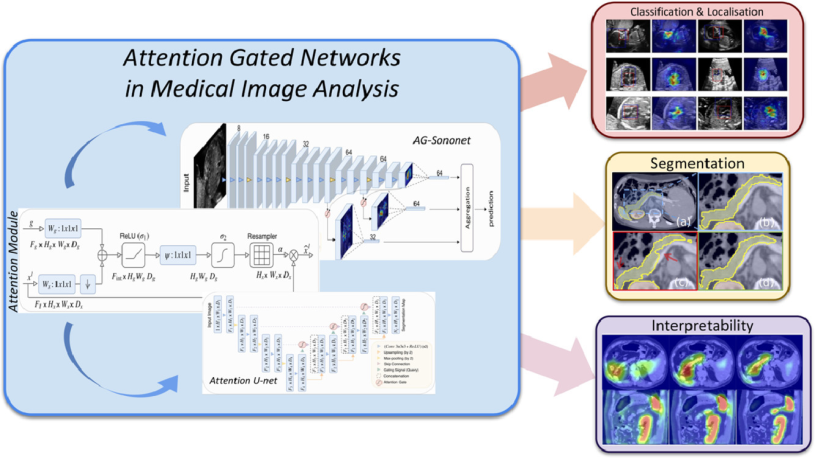
You can imagine heatmaps are also applied in medical imaging to comprehend the area of interest that the neural network uses to make the decision. They use gradients from a pre-trained neural network to produce a coarse localization map highlighting the vital regions of the image for predicting the image’s classification. For example, the heatmap is used to detect the blood patterns in the hemophilia knee ultrasound images to help doctors diagnose hemarthrosis.

Now on to the fun part, using Heatmap in a sentence by the end of the day! (See rules here)

Serious: We use heatmaps to check whether the model is detecting the domain of interest. 

Less serious: * On the road“Which way should we go next?” “Right side! There are fewer people than the left side.” “How do you know?” “Heatmap said!”

… I’ll see you in the blogosphere.

Qianyu Fan

Qianyu Fan’s ROP299 Experience

My name is Qianyu Fan, and I finished my first year at the University of Toronto, pursuing a statistics specialist. This summer I was given the incredible opportunity to work in Dr. Tyrrell’s lab for the ROP299 course. These four months, I have gone through pain and suffering, underwent a metamorphosis, and finally reaped the fruits.

I still remembered that I promised Professor Tyrrell during the interview that I would put twice as much effort as others to complete scientific research. Even if I had no experience with machine learning and neural networks, even if I hadn’t heard of them, the professor was welcome to accept me! During the weekly meetings, terminologies were hard for me to understand, though I tried to research them afterward. And so, I began my research in a daze.

Early on, I floundered to find a focus. The topic “Compare Image Similarity” is huge, where I could do the research on many sides. For instance, we could use different distance metrics to explore the similarities between synthetic and real images. Also, whether replacing real with synthetic images will improve the model accuracy in the training process is a meaningful topic. Due to many interesting ideas for the project, I was lost, and the proposal had been constantly revised. As other ROP students were starting to write their projects, I was still stuck in the proposal and was anxious about the progress. The professor understood my situation and helped me redefine my direction, because he cared about what the students learned in the course. So, my theme was: Comparison of Two Augmentation Methods in Improving Detection Accuracy of Hemarthrosis. We used data synthesis and traditional augmentation techniques to explore and compare the recognition accuracy with increasing proportions of augmented data.

As the deadline was approaching, I had the idea of giving up due to no results. Once in the private meeting with the professor, I broke down and cried. What a shame! He gave me much support and understood my frustration. Mauro was very helpful in offering the datasets as well as allowing me to use his codes and solving my questions. Thanks to their help, my thinking became clear, and I was able to complete the project on time.

A tortuous but unforgettable journey is over. I have learned a lot of things in this ROP course, from machine learning to scientific research. This will be an asset in my life. I appreciate that the professor gave me this opportunity and that I was able to complete my project.

Qianyu Fan

Jenny Du’s ROP299 Journey: Telling apart the real and the fake!

My name is Jenny Du, and I have just wrapped up my ROP299 project in the Tyrrell Lab, as well as my second year at the University of Toronto, pursuing a bioinformatics specialist. Looking back, it was a bumpy ride, but in the end, this journey was very rewarding and has taught me a lot of things on both machine learning topics as well as the process of scientific research.

Like most of the other ROP299 students, I had no experience with machine learning and neural networks. Despite doing some research beforehand, I found myself googling what everyone was talking about during the weekly meetings (thankfully, they were online) to make sure I was not completely lost. None of my first-year courses had prepared me for these kinds of things! And so, with some uncertainties in my heart, I started my ROP journey.

I decided on my overall research topic fairly early, but the details were adjusted several times as I progressed through my project. My project is about coming up with a way to quantitatively assess a set of synthetic ultrasound images in terms of how “realistic” they look compared to the real ultrasound images. “Realism” here is defined as whether the synthetic images can be used as training images in replacement of the real images without creating too big of an impact on the machine learning algorithm. At first, I came up with a naïve proposal: I will build an algorithm that differentiates real and synthetic ultrasound images, and if the algorithm can classify the two kinds (with high accuracies), then it means that the synthetic images are not realistic, and vice versa. In the weekly meeting, Dr. Tyrrell immediately pointed out why this wouldn’t work. In my proposal, a low accuracy could mean that the synthetic and the real images are very similar, but it could also mean that the algorithm itself is terrible. For example, if my algorithm has 50% accuracy, then it is basically randomly guessing each image, like a coin toss, so its classification is unreliable, to say the least. He suggested that I look online to see how others have done it. There was very little information that directly relates to what I’m doing, but eventually I was able to come up with a plan to extract features from the images using a pre-trained CNN model and measure the cosine similarity score between two images and graph these values into a histogram to see their distribution. Dr. Tyrrell also suggested that I compare the distributions at different equivalence margins to determine how big a mean difference is acceptable.

Thankfully, I was able to find some code online that I was able to use in my project with minor changes, and I was able to produce some distribution data fairly quickly. Then, I encountered what I considered to be the hardest part of my entire project: to statistically interpret and discuss my data and create a conclusion out of it. Since I am not a statistics student, and so my knowledge of statistics is limited to one stats course I took as a part of my program requirements. It took a while for me to learn all these statistical concepts and understand why each is needed in my project.

This year was especially interesting since everything was online. Despite not being able to see each other face-to-face, I was still able to receive much support from Dr. Tyrrell and other students in the lab. Mauro was very helpful in preparing the datasets for my project as well as answering any problems related to the codes. Guan also helped to check my statistical calculations and clarifying some hard concepts. I have also made great friends with the other ROP students this year, and hopefully we will be able to see each other in person when the school re-opens.

Overall, this journey was a wonderful experience, and I have learned many things from it. Not only did I got some familiarity with machine learning topics and their application in medicine, but I have also gained experience in the general academic research process, from coming up with a topic to the actual implementation to the final reports. There were challenges along the way, but in the end, it was very rewarding. I am extremely thankful to Dr. Tyrrell for the guidance and support and am grateful for this opportunity.

Jenny Du

MiWORD of the Day Is…Cosine Distance!

            Today we will talk about a way to measure distance, but not about how far away two objects are. Instead, cosine distance, or cosine similarity, is a measure of how similar two non-zero vectors are in terms of orientation, or to put it simply, the direction to which they point. Mathematically, the cosine similarity between two 2-D vectors is equal to the cosine of the angle between them, which can also be calculated using their dot product and magnitudes, as shown on the right. Two vectors pointing in the same direction will have a cosine similarity of 1; two vectors perpendicular to each other will have a similarity of 0; two vectors pointing in opposite direction will have a similarity of -1. Cosine distance is equal to (1 – cosine similarity). In this case, two vectors will have a cosine distance between 0 to 2: 0 when they are pointing in the same direction, and 2 when they are pointing in opposite direction. Cosine similarity and distance essentially measure the same thing, but the distance will convert any negative values to positive.

           Cosine distance and similarity also apply to higher dimensions, which makes them useful in analyzing images, texts, and other forms of data. In machine learning, we can use an algorithm to process a dataset of information and store each object as an array of multidimensional vectors, where each vector represents a feature. Then, we can use cosine similarity to compare how similar each pair of vectors are between the two objects and come up with an overall similarity score. In this case, two identical objects will have a similarity score of 1. In higher dimensions, we can rely on the computer to do the calculations for us. For example, we have the distance.cosine function in the SciPy package in Python will compute the cosine distance between two vector arrays in one go.

Here are two examples of how you can use cosine distance in a conversation:

Serious:  “I copied an entire essay for my assignment and this online plagiarizing checker says my similarity score is only 1! Time to hand it in.” “It says a COSINE similarity of 1. Please go back and write it yourself…”

Less serious: *during a police car chase* “Check how far are we from the suspect’s car!” “Well, assuming that he doesn’t turn, the distance between us will always be zero. Remember from your math class? Two vectors pointing in the same direction will always have a cosine distance of zero…”

… I’ll see you in the blogosphere.

Jenny Du

Parinita Edke’s ROP experience in the Tyrrell Lab!

Hi! My name is Parinita Edke and I’m finishing my third year at UofT, specializing in Computer Science with a minor in Statistics. I did a STA399Y research project with Professor Tyrrell from September 2020 – April 2021 and I am excited to share my experience in the lab!

I have always been interested in medicine and the applications of Computer Science and Statistics to solve problems in the medical field. I was looking out for opportunities to do research in this intersection and was excited when I saw Professor Tyrrell’s ROP posting. I applied prior to the second-round deadline and waited to hear back. After almost 2 weeks past the deadline, I had still not heard back and decided to follow up on the status of my application. I quickly received a reply from Professor Tyrrell that he had already picked his students prior to receiving my application. While this was extremely disappointing, I thanked Professor Tyrrell for his time and expressed that I was still interested in working with him during the year and attached my application package to the email. I was not really expecting anything coming out of this, so I was extremely happy when I received an invite to an interview! After a quick chat with Professor Tyrrell about my goals and fit for the lab, I was accepted as an ROP student!

Soon after being accepted, I joined my first lab meeting where I was quickly lost in the technical machine learning terms, the statistical concepts and the medical imaging terminology used. I ended the meeting determined to really begin understanding what machine learning was all about!

This marked the beginning of the long and challenging journey through my project. When I decided on my project, it seemed interesting as solving the problem allowed for some cool questions to be answered. The task was to detect the presence of blood in ultrasound images of the knee joint; my project was to determine if Fourier Transformation can be used to generate features to perform the task at hand well. It seemed quite straightforward at first – simply generate Fourier Transformed features and run a classification model to get the outputs, right? After completing the project, I am here to tell you that it was far from being straightforward. It was more like a zigzag progress pattern through the project. The first challenge that I faced was understanding the theory behind the Fourier Transform and how it applies to the task at hand. This took me quite some time to fully grasp and was definitely one of the more challenging parts of the project. The next challenge was figuring out the steps and the things I would need for my project. Rajshree, a previous lab member, had done some initial work using a CNN+SVM model. I first tried to replicate what Rajshree had done in order to create a baseline to compare my approach to. It took me some time to understand what each line of code did within Rajshree’s model but after I was able to get it to work, I felt amazing! Reading through Rajshree’s code gave me more experience in understanding the common Python libraries used in machine learning, so when I built my model, it was much quicker! When I ran my model for the first time, I felt incredible! The process was incredibly frustrating at times, but when I saw results for the first time, I felt like all this struggle was worth it. Throughout this process of figuring out the project steps and building the model, Mauro was always there to help, always being enthusiastic when answering any questions I had and giving me encouragement to keep going.

Throughout the process, Professor Tyrrell was always there as well – during our weekly ROP meetings, he always reminded us to think about the big picture of what our projects were about and the objectives we were trying to accomplish. I definitely veered off in the wrong direction at times, but Professor Tyrrell was quick to pull me back and redirect me in the right direction. Without this guidance, I would not have been able to finish and execute the project in the way that I did and am proud of.

Looking back at the year, I am astonished at the number of things I have learned and how much I have grown. Everything that I learned, not only about machine learning, but about writing a research paper, learning from others and your own mistakes, collaborating with others, learning from even more of my own mistakes, and persevering when things get tough will carry with me throughout the rest of my undergraduate studies and the rest of my professional career.

Thank you, Professor Tyrrell, for taking a chance on me. He could have simply passed on my application but the fact that he took a chance with me and accepted me into the course lead to such an invaluable experience for me which I truly appreciate. The experiences and the connections I have made in this lab have been a highlight of my year, and I hope to keep contributing to the lab in the future!

Parinita Edke

MiWord of the Day Is… Fourier Transform!

Ok, a what Transform now??

In the early 1800s, Jean-Baptiste Joseph Fourier, a French mathematician and physicist, introduced the transform in his study of heat transfer. The idea seemed preposterous to many mathematicians at the time, but it has now become an important cornerstone in mathematics.

So, what exactly is the Fourier Transform? The Fourier Transform is a mathematical transform that decomposes a function into its sine and cosine components. It decomposes a function depending on space or time into a function depending on spatial or temporal frequency.

Before diving into the mathematical intricacies of the Fourier Transform, it is important to understand the intuition and the key idea behind it. The main idea of the Fourier Transform can be explained simply using the metaphor of creating a milkshake.

Imagine you have a milkshake. It is hard to look at a milkshake and understand it directly; answering questions such as “What gives this shake its nutty flavour?” or “What is the sugar content of this shake?” are harder to answer when we are simply given the milkshake. Instead, it is easier to answer these questions by understanding the recipe and the individual ingredients that make up the shake. So, how exactly does the Fourier Transform fit in here? Given a milkshake, the Fourier Transform allows us to find its recipe to determine how it was created; it is able to present the individual ingredients and the proportions at which they were combined to make the shake. This brings up the questions of how does the Fourier transform determine the milkshake “recipe” and why would we even use this transform to get the “recipe”? To answer the former question, we are able to determine the recipe of the milkshake by running it through filters that then extract each individual ingredient that makes up the shake. The reason we use the Fourier Transform to get the “recipe” is that recipes of milkshakes are much easier to analyze, compare, and modify than working with the actual milkshake itself. We can create new milkshakes by analyzing and modifying the recipe of an existing milkshake. Finally, after deconstructing the milkshake into its recipe and ingredients and analyzing them, we can simply blend the ingredients back to get the milkshake.

Extending this metaphor to signals, the Fourier Transform essentially takes a signal and finds the recipe that made it. It provides a specific viewpoint: “What if any signal could be represented as the sum of simple sine waves?”.

By providing a method to decompose a function into its sine and cosine components, we can analyze the function more easily and create modifications as needed for the task at hand.

 A common application of the Fourier Transform is in sound editing. If sound waves can be separated into their “ingredients” (i.e., the base and treble frequencies), we can modify this sound depending on our requirements. We can boost the frequencies we care about while hiding the frequencies that cause disturbances in the original sound. Similarly, there are many other applications of the Fourier Transform such as image compression, communication, and image restoration.

This is incredible! An idea that the mathematics community was skeptical of, now has applications to a variety of real-world applications.

Now, for the fun part, using Fourier Transform in a sentence by the end of the day:

Example 1:

Koby: “This 1000 puzzle is insanely difficult. How are we ever going to end up with the final puzzle picture?”

Eng: “Don’t worry! We can think of the puzzle pieces as being created by taking the ‘Fourier transform’ of the puzzle picture. All we have to do now is take the ‘inverse Fourier Transform’ and then we should be done!”

Koby: “Now when you put it that way…. Let’s do it!”

Example 2: 

Grace: “Hey Rohan! What’s the difference between a first-year and fourth-year computer science student?

Rohan: “… what?”

Grace: “A Fouri-y-e-a-r Transform”

Rohan: “…. (╯°□°)╯︵ ┻━┻ ”

I’ll see you in the blogosphere…

Parinita Edke

The MiDATA Word of the Day is…”clyster”

Holy mother of pearl! Do you remember when the first Pokémon games came out on the Game Boy? Never heard of Pokémon? Get up to speed by watching this short video. Or even better! Try out one of the games in the series, and let me know how that goes!

The name of the Pokémon in this picture is Cloyster. You may remember it from Pokémon Red or Blue. But! Cloyster, in fact, has nothing to do with clysters.

In olden days, clyster meant a bunch of persons, animals or things gathered in a close body. Now, it is better known as a cluster.

You yourself must identify with at least one group of people. What makes you human; your roles, qualities, or actions make you unique. But at the same time, you fall into a group of others with the same characteristics.

You yourself fall into multiple groups (or clusters). This could be your friend circle or perhaps people you connect with on a particular topic. At the end of the day, you belong to these groups. But is there a way we can determine that you, in fact, belong?

Take for example Jack and Rose from the Titanic. Did Jack and Rose belong together?

If you take a look at the plot to the right, Jack and Rose clearly do not belong together. They belong to two separate groups (clusters) of people. Thus, they do not belong together. Case closed!

But perhaps it is a matter of perspective? Let’s take a step back…

Woah! Now, you could now say that they’re close enough, they might as well be together! Compared to the largest group, they are more similar than they are different. And so, they should be together!

For the last time, we may have been looking at this completely wrong! From the very beginning, what are we measuring on the x-axis and on the y-axis of our graph?

Say it was muscle mass and height. That alone shouldn’t tell us if Rose and Jack belong together! And yet, that is exactly what we could have done. But if not those, then what..?

Now for the fun part (see the rules here), using clyster in a sentence by the end of the day:

Serious: Did you see the huge star clysters last night? I heard each one contained anywhere from 10,000 to several million stars…

Less serious: *At a seafood restaurant by the beach* Excuse me, waiter! I’d like one of your freshest clysters, please. – “I’m sorry. We’re all out!”

…I’ll see you in the blogosphere.

Stanley Hua

Stanley Hua in ROP299: Joining the Tyrrell Lab during a Pandemic

My name is Stanley Hua, and I’ve just finished my 2nd year in the bioinformatics program. I have also just wrapped up my ROP299 with Professor Pascal. Though I have yet to see his face outside of my monitor screen, I cannot begin to express how grateful I am for the time I’ve been spending at the lab. I remember very clearly the first question he asked me during my interview: “Why should I even listen to you?” Frankly, I had no good answer, and I thought that the meeting didn’t go as well as I’d hoped. Nevertheless, he gave me a chance, and everything began from there.

Initially, I got involved with quality assessment of Multiple Sclerosis and Vasculitis 3D MRI images along with Jason and Amar. Here, I got introduced to the many things Dmitrii can complain about taking brain MRI images. Things such as scanner bias, artifacts, types of imaging modalities and prevalence of disease play a role in how we can leverage these medical images in training predictive models.

My actual ROP, however, revolved around a niche topic in Mauro and Amar’s project. Their project sought to understand the effect of dataset heterogeneity in training Convolutional Neural Networks (CNN) by cluster analysis of CNN-extracted image features. Upon extraction of image features using a trained CNN, we end up with high-dimensional vectors representing each image. As a preprocessing step, the dimensionality of the features is reduced by transformation via Principal Component Analysis, then selecting a number of principal components (PC) to keep (e.g. 10 PCs). The question must then be asked: How many principal components should we use in their methodology? Though it’s a very simple question, I took way too many detours to answer this question. I looked at the difference between standardization vs. no standardization before PCA, nonlinear dimensionality reduction techniques (e.g. autoencoder) and comparisons of neural network image representation (via SVCCA) among other things. Finally, I proposed an equally simple method for determining the number of PCs to use in this context, which is the minimum number of PCs that gives the most frequent resulting value (from the original methodology).

Regardless of the difficulty of the question I sought to answer, I learned more about practices in research, and I even learned about how research and industry intermingle. I only have Professor Pascal to thank for always explaining things in a way that a dummy such as me would understand. Moreover, Professor Pascal always focused on impact; is what you’re doing meaningful and what are its applications?

 I believe that the time I spent with the lab has been worthwhile. It was also here that I discovered that my passion to pursue data science trumps my passion to pursue medical school (big thanks to Jason, Indranil and Amar for breaking my dreams). Currently, I look towards a future, where I can drive impact with data; maybe even in the field of personalized medicine or computational biology. Whoever is reading this, feel free to reach out! Hopefully, I’ll be the next Elon Musk by then…

Transiently signing out,

Stanley Bryan Z. Hua

Jessica Xu’s Journey in ROP299

Hello everyone! My name is Jessica Xu, and I’ve just completed my second year in Biochemistry and Statistics at the University of Toronto. This past school year, I’ve had the wonderful opportunity to do a ROP299 project with Dr. Pascal Tyrrell and I’d like to share my experience with you all!

A bit about myself first: in high school, I was always interested in life sciences. My favourite courses were biology and chemistry, and I was certain that I would go to medical school and become a doctor. But when I took my first stats course in first year, I really enjoyed it and I started to become interested in the role of statistics in life sciences. Thus, at the end of my first year, while I was looking through the various ROP courses, I felt that Dr. Tyrrell’s lab was the perfect opportunity to explore my budding interest in this area. I was very fortunate to have an interview with Dr. Tyrrell, and even more fortunate to be offered a position in his lab!

Though it may be obvious, doing a research project when you have no research experience is very challenging! Coming into this lab having taken a statistics course and a few computer science courses in first year, I felt I had a pretty good amount of background knowledge. But as I joined my first lab meeting, I realized I couldn’t be more wrong! Almost every other word being said was a word I’d never heard of before! And so, I realized that there was a lot I needed to learn before I could even begin my project.

I then began on the journey of my project, which was looking at how two dimension reduction techniques, LASSO and SES, performed in an ill-posed problem. It was definitely no easy task! While I had learned a little bit about dimension reduction in my statistics class, I still had a lot to learn about the specific techniques, their applications in medical imaging, and ill-posed problems. I was also very inexperienced in coding, and had to learn a lot of R on my own, and become familiar with the different packages that I would have to use. It was a very tumultuous journey, and I spent a lot of time just trying to get my code to work. Luckily, with help from Amar, I was able to figure out some of the errors and issues I was facing in regards to the code.

I learned a lot about statistics and dimension reduction in this ROP, more than I have learned in any other courses! But most importantly, I had learned a lot about the scientific process and the experience of writing a research paper. If I can provide any advice based on my experience, it’s that sometimes it’s okay to feel lost! It’s not expected of you to have devised a perfect plan of execution for your research, especially when it’s your first time! There will be times that you’ll stray off course (as I often did), but the most valuable lesson that I learned in this ROP is how to get back on track. Sometimes you just need to take a step back, go back to the beginning and think about the purpose of your project and what it is you’re trying to tell people. But it’s not always as easy to realize this. Luckily Dr. Tyrrell has always been there to guide us throughout our projects and to make sure we stay on track by reminding us of the goal of our research. I’m incredibly grateful for all the support, guidance, and time that Dr. Tyrrell has given this past year. It has been an absolute pleasure of having the experience of working in this lab.

Now that I’ve taken my first step into the world of research, with all the new skills and lessons I’ve learned in my ROP, I look forward to all the opportunities and the journey ahead!

Jessica Xu

Today’s MiWORD of the day is… Lasso!

Wait… Lasso? Isn’t a lasso that lariat or loop-like rope that cowboys use? Or perhaps you may be thinking about that tool in Photoshop that’s used for selecting free-form segments!

Well… technically neither is wrong! However, in statistics and machine learning, Lasso stands for something completely different: least absolute shrinkage and selection operator. This term was coined by Dr. Robert Tibshirani in 1996 (who was a UofT professor at that time!).

Okay… that’s cool and all, but what the heck does that actually mean? And what does it do?

Lasso is a type of regression analysis method, meaning it tries to estimate the relationship between predictor variables and outcomes. It’s typically used to perform feature selection or regularization.

Regularization is a way of reducing overfitting of a model, ie. it removes some of the “noise” and randomness of the data. On the other hand, feature selection is a form of dimension reduction. Out of all the predictor variables in a dataset, it will select the few that contribute the most to the outcome variable to include in a predictive model.

Lasso works by applying a fixed upper bound to the sum of absolute values of the coefficient of the predictors in a model. To ensure that this sum is within the upper bound, the algorithm will shrink some of the coefficients, particularly it shrinks the coefficients of predictors that are less important to the outcome. The predictors whose coefficients are shrunk to zero are not included at all in the final predictive model.

Lasso has applications in a variety of different fields! It’s used in finance, economics, physics, mathematics, and if you haven’t guessed already… medical imaging! As the state-of-the-art feature selection technique, Lasso is used a lot in turning large radiomic datasets into easily interpretable predictive models that help researchers study, treat, and diagnose diseases.

Now onto the fun part, using Lasso in a sentence by the end of the day! (see rules here)

Serious: This predictive model I got using Lasso has amazing accuracy for detecting the presence of a tumour!

Less serious: I went to my professor’s office hours for some help on how to use Lasso, but out of nowhere he pulled out a rope!

See you in the blogosphere!

Jessica Xu