Who’s in Agreement?

So, let’s say you have invited everyone over for the big game on Sunday (Superbowl 49) but you don’t have a big screen TV. Whoops! That sucks. Time to go shopping. Here’s the rub: which one to get? There are so many to chose from and only a little time to make the decision. Here is what you do:


1- call your best friends to help you out
2- make a list of all neighboring electronics stores 
3- Go shopping!


OK, that sounds like a good plan but it will take an enormous amount of time to perform this task all together and more importantly your Lada only seats 4 comfortably and you are 8 buddies.


As you are a new research scientist (see here for your story) and you have already studied the challenges of assessing agreement (see here for a refresher) you know that it is best for all raters to assess the same items of interest. This is called a fully crossed design. So in this case you and all of your friends will assess all the TVs of interest. You will then make a decision based on the ratings. Often, it is of interest to know and to quantify the degree of agreement between the raters – your friends in this case. This assessment is the inter-rater reliability (IRR). 


As a quick recap, 


Observed Scores = True Score + Measurement Error


And


Reliability = Var(True Score)/ Var(True Score) + Var(Measurement Error)


Fully crossed designs allow you to assess and control for any systematic bias between raters at the cost of an increase in the number of assessments made. 


The problem today is that you want to minimize the number of assessments made in order to save time and keep your buddies happy. What to do? Well, you will simply perform a study where different items will be rated by different subsets of raters. This is a “not fully crossed” design! 


However, you must be aware that with this type of design you are at risk of underestimating the true reliability and therefore must, therefore, perform alternative statistics.


I will not go into statistical detail (today anyway!) but if you are interested have a peek here. The purpose of today’s post was simply to bring to your attention that you need to be very careful when assessing agreement between raters when NOT performing a fully crossed design. The good news is that there is a way to estimate reliability when you are not able to have all raters assess all the same subjects.


Now you can have small groups of friends who can share the task of assessing TVs. This will result in less assessments, less time to complete the study, and – most importantly – less use of your precious Lada! 


Your main concern, as you are the one to make the purchase of the TV, is still: can you trust your friends assessment score of TVs you did not see? But now you have a way to determine if you and your friends are on the same page!


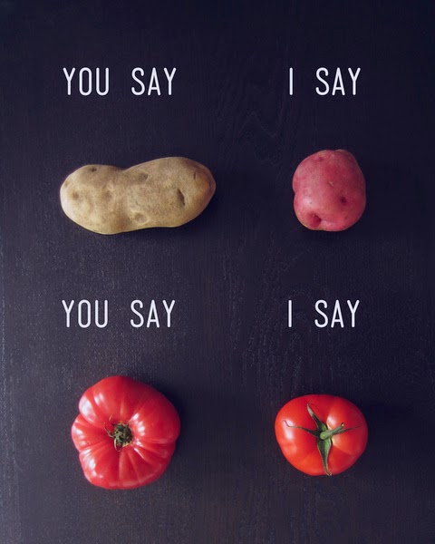
Maybe this will avoid you and your friends having to Agree to Disagree as did Will Ferrell in Anchorman…


Listen to an unreleased early song by Katy Perry Agree to Disagree, enjoy the Superbowl (and Katy Perry) on Sunday and…


…I’ll see you in the blogosphere!


Pascal Tyrrell

Who is your neighbor?

Classic Seth Rogan movie. Today we will be talking about good neighbors as a followup to my first post “What cluster Are You From?“. If you want to learn a little about bad neighbors watch the trailer to the movie Neighbors.


So let’s say you are working with a large amount of data that contains many, many variables of interest. In this situation you are most likely working with a multidimensional model. Multivariate analysis will help you make sense of multidimensional space and is simply defined as a situation when your analysis incorporates more than 1 dependent variable (AKA response or outcome variable). 


*** Stats jargon warning*** 
Mulitvariate analysis can include analysis of data covariance structures to better understand or reduce data dimensions (PCA, Factor Analysis, Correspondence Analysis) or the assignment of observations to groups using a unsupervised methodology (Cluster Analysis) or a supervised methodology (K Nearest Neighbor or K-NN). We will be talking about the later today.


*** Stats-reduced safe return here***
Classification is simply the assignment of previously unseen entities (objects such as records) to a class (or category) as accurately as possible.  In our case, you are fortunate to have a training set of entities or objects that have already been labelled or classified and so this methodology is termed “supervised”. Cluster analysis is unsupervised learning and we will talk more about this in a later post.


Let’s say for example you have made a list of all of your friends and labeled each one as “Super Cool”, “Cool”, or “Not cool”. How did you decide? You probably have a bunch of attributes or factors that you considered. If you have many, many attributes this process could be daunting. This is where k nearest neighbor or K-NN comes in. It considers the most similar other items in terms of their attributes, looks at their labels, and gives the unassigned object the majority vote!


This is how it basically works:


1- Defines similarity (or closeness) and then, for a given object, measures how similar are all the labelled objects from your training set. These become the neighbors who each get a vote.


2- Decides on how many neighbors get a vote. This is the k in k-NN.


3- Tallies the votes and voila – a new label! 


All of this is fun but will be made much easier using the k-NN algorithm and your trusty computer!


So, now you have an idea about supervised learning technique that will allow you to work with a multidimensional data set. Cool.


Listen to Frank Sinatra‘s The Girl Next Door to decompress and I’ll see you in the blogosphere…


Pascal Tyrrell

What Cluster Are You From?

This week and I had the pleasure of presenting to the Division of Rheumatology Research Rounds – University of Toronto. They were a fantastic audience who asked questions and appeared to be very engaged. Shout out to the Rheumatology gang!


So, I was asked to talk about a statistical methodology called Cluster Analysis. I thought I would start a short series on the topic for you guys. Don’t worry I will keep the stats to a minimum as I always do!


Complex information can always be best recognized as patterns. The first picture below on the left certainly helps you realize that it is not a simple task to know someone at a glance.


Now, I guess it doesn’t help that many of you have never met me either! However, you can appreciate that things get a little easier when the same portrait is presented in the usual manner – upright! 


This is an interesting example where the information is identical, however, our ability to intuitively recognize a pattern (me!) appears to be restricted to situations that we are familiar with.


This intuition often fails miserably when abstract magnitudes (numbers!) are involved. I am certain most of us can relate to that. 


The good news is that with the advent of crazy powerful personal computers we can benefit from complex and resource intensive mathematical procedures to help us make sense of large scary looking data sets.


So, when would you use this kind of methodology you ask? I’ll tell you…


1 – Detection of subgroups/ clusters of entities (ie: items, subjects, users…) within your data set.


2 – Discovery of useful, possibly unexpected, patterns in data.


OK, time for some homework. Try to think of times when you could apply this kind of analysis. 


I’ll start you off with an example that you can relate to. Every time you go to YouTube and search for your favorite movie trailer you get a long list of other items on the right that YouTube thinks may be of interest to you. How do you think they do that? By taking into account things like keywords, popularity, and user browser history (and many, many more variables) and using cluster analysis of course! You and your interests belong to a cluster. Cool!


In this series, we will delve into this fun world of working with patterns in data. 


Now that you have peace of mind, listen to The Grapes of Wrath


See you in the blogosphere,


Pascal Tyrrell


Face Validity: Who’s Face Is It Anyway?

Yes, I was a big fan of the A-Team. Who wasn’t? Mr. T (I guess that makes me Prof. T…) was always entertaining to watch. Lieutenant Templeton Arthur Peck was suave, smooth-talking, and hugely successful with women. Peck served as the team’s con man and scrounger, able to get his hands on just about anything they needed. Need a refresher? Have a peek here.


Well in a past post 2 Legit 2 Quit we talked about why we assess validity – because we want to know the nature of what is being measured and the relationship of that measure to its scientific aim or purpose. So what if we are uncertain that our measure (a scale for example) looks reasonable? We would consider face validity and content validity. Essentially, face validity assess whether or not the instrument we are using to measure appears to be assessing the desired qualities or attributes based on “the face of it”. Content validity – that was touched on in the previous post – is closely related and considers whether the instrument samples all of the relevant or important content or interest.


So, why the importance of face validity? Whenever you need to interact successfully with study participants there is often a need to:


– increase motivation and cooperation from participants for better responses.
– attract as many potential candidates.
– reduce dissatisfaction among users.
– make your results more generalizable and appealing to stake holders.


These are especially important points to consider when planning a study that involves human subjects as respondents or there exists any level of subjectivity in how data is collected for the variables of interest in your study. 


However, you want to avoid a “Con Man” situation in your study where respondents’ answers are not what they appear to be. As a researcher you need to be aware that there may be situations where Face Validity may not be achievable. Let’s say for instance you are interested in discovering all factors related to bullying in high school. If you were to ask the question ‘ have you ever bullied a classmate into given you his/her lunch money?’ you may have Face Validity but you may not get an honest response! In this case, you may consider a question that does not have face validity but will elicit the wanted answer. Ultimately, the decision on whether or not to have face validity – where the meaning and relevance are self-evident – depends on the nature and purpose of the instrument. Prepare to be flexible in your methodology!


Remember that face validity pertains to how your study participants perceive your test. They should be the yard stick by which you assess whether you have face validity or not.


Listen to Ed Sheeran – The A Team to decompress and…


… I’ll see you in the blogosphere.


Pascal Tyrrell

Breaking Up Is Hard to Do

Last week I met with Helen, a clinical investigator program radiology resident from our department, about her research (shout out to Dr Laurent Milot’s research group). When discussing predictors and outcomes for her retrospective study it was suggested that some continuous variables be broken up into levels or categories based on given cut-points. This practice is often encountered in the world of medical research. The main reason? People in the medical community find it easier to understand results that are expressed as proportions, odds ratio, or relative risk. When working with continuous variables we end up talking about parameter estimates / beta weights and such – not as “reader friendly”. 


Unfortunately, as Neil Sedaka sang about in his famous song Breaking Up Is Hard to Do, by breaking up continuous variables you pay a stiff penalty when it comes to your ability to describe the relationship that you are interested in and the sample size requirements (see loss of power) of your study.


You are now a newly minted research scientist (need a refresher? See Pocket Protector) and are interested in discovering relationships among variables or between predictors and outcomes. The more accurate your findings the better the description of the relationships and the better the interpretation/ conclusions you can make.The bottom line is that dichotomizing/ categorizing a continuous measure will result in loss of information. Essentially, the “signal” which is the information captured by your measure will be reduced by categorization and, therefore, when you perform a statistical test that compares this signal to the “noise” or error of the model (observed differences between your patients for example) you will find yourself at a disadvantage (loss of power)David Streiner (great author and great guy!) gives a more complete explanation in one of his papers.


Now, as we see in the funny movie with Vince Vaugh and Jennifer Aniston, The Break Up, there are times when categorization may make sense. For example when the variable you are considering is not normally distributed (see Are You My Type?) or when the relationship that you are studying is not linear. We will talk about these situations in a later post.


Don’t forget: you will get further ahead if you keep your variables as continuous data whenever possible.


See you in the blogosphere,


Pascal Tyrrell

You like potato and I like potahto… Let’s Call the Whole Thing Off!

We have been talking about agreement lately (not sure what I am talking about? See the start of the series here) and we covered many terms that seem similar. Help!


Before you call the whole thing off and start dancing on roller skates like Fred Astaire and Ginger Roberts did in Shall We Dance, let’s clarify a little the difference between agreement and reliability. 


When assessing agreement in medical research, we are often interested in one of three things:


1- comparing methods – à la Bland and Altman style.


2- validating an assay or analytical method.


3- assessing bioequivalence.


Agreement represents the degree of closeness between readings. We get that. Now reliability on the other hand actually assesses the degree of differentiation between subjects – so one’s ability to tell subjects apart from within a population. Yes, I realize this is a subtlety just as Ella Fitzgerald and Louis Armstrong sing about in the original Let’s Call the Whole Thing Off.


Now, often when assessing agreement one will use an unscaled index (ie a continuous measure for which you calculate the Mean Squared Deviation, Repeatability Standard Deviation, Reproducibility Standard Deviation, or the Bland and Altman Limits of Agreement) whereas when assessing reliability one often uses a scaled index (ie a measure for which you can calculate the Intraclass Correlation Coefficient or Concordance Correlation Coefficient). This is because a scaled index mostly depends on between-subject variability and, therefore, allows for the differentiation of subjects from a population. 


Ok – clear as mud. Here are some very basic guidelines:


1- Use descriptive stats to start with.


2- Follow it up with an unscaled index measure like the MSD or LOI which deal with absolute values (like the difference).


3- Finish up with a scaled index measure that will yield a standardized value between -1 and +1 (like the ICC or CCC).


Potato, Potahtoe. Whatever. 


Entertain yourself with this humorous clib from the Secret Policeman’s Ball and I’ll…

See you in the blogosphere!


Pascal Tyrrell

2 Legit 2 Quit

MC Hammer. Now those were interesting pants! Heard of the slang expression “Seems legit”? Well “legit” (short for legitimate) was popularized my MC Hammer’s song 2 Legit 2 Quit. I had blocked the memories of that video for many years. Painful – and no I never owned a pair of Hammer pants!


Whenever you sarcastically say “seems legit” you are suggesting that you question the validity of the finding. We have been talking about agreement lately and we have covered precision (see Repeat After Me), accuracy (see Men in Tights), and reliability (see Mr Reliable). Today let’s cover validity.


So, we have talked about how reliable a measure is under different circumstances and this helps us gauge its usefulness. However, do we know if what we are measuring is what we think it is. In other words, is it valid? Now reliability places an upper limit on validity – the higher the reliability, the higher the maximum possible validity. So random error will affect validity by reducing reliability whereas systematic error can directly affect validity – if there is a systematic shift of the new measurement from the reference or construct. When assessing validity we are interested in the proportion of the observed variance that reflects variance in the construct that the method was intended to measure.


***Too much stats alert*** Take a break and listen to Ice, Ice, Baby from the same era as MC Hammer and when you come back we will finish up with validity. Pants seem similar – agree? 🙂


OK, we’re back. The most challenging aspect of assessing validity is the terminology. There are several different types of validity dependent of the type of reference standard you decide to use (details to follow in later posts):


1- Content:  the extent to which the measurement method assesses all the important content.


2- Construct: when measuring a hypothetical construct that may not be readily
observed.


3- Convergent: new measurement is correlated with other measurements of the same construct.


4- Discriminant: new measurement is not correlated with unrelated constructs.

So why do we assess validity? because we want to know the nature of what is being measured and the relationship of that measure to its scientific aim or purpose.


I’ll leave you with another “seem legit” picture that my kids would appreciate…


See you in the blogosphere,


Pascal Tyrrell


Mr Reliable

Kevin Durant is Mr Reliable

Being reliable is an important and sought after trait in life. Kevin Durant has proven himself to be just that to the NBA. Would you agree (pun intended)? So, we have been talking about agreement lately and we have covered precision (see Repeat After Me) and accuracy (see Men in Tights). Today let’s talk a little about reliability.

 
As I mentioned last time, the concepts of accuracy and precision originated in the physical sciences because direct measurements are possible. Not to be outdone, the social sciences (and later in the Medical Sciences) decided to define their own terms of agreement – validity and reliability.
 
So the concept of reliability was developed to reflect the amount of error, both random and systematic, in any given measurement. For example if you were to want to assess the the measurement error in repeated measurements on the same subject under identical conditions or to measure the consistency of two readings obtained by two different readers on the same subject under identical conditions. 
 
The reliability coefficient is simply the ratio of variability between subjects to the total variability (sum of subject variability and measurement error). A coefficient of 0 indicates no reliability and 1 indicates perfect reliability with no measurement error.
 
Being Mr Reliable (see the trailer to this cool old movie from the sixties) is always desirable but keep in mind that when you consider reliability remember that:
 
1- A true score exists but is not directly measurable (philosophical…)
 
2- A measurement is always the sum of the true score and a random error.
 
3- Any two measurements for the same subject are parallel measurements in that they are assumed to have the same mean and variance.
 
 
With these assumptions in place, reliability can be also expressed as the correlation between any two measurements on the same subject – AKA the intraclass correlation coefficient or ICC (originally defined by Sir Francis Galton and later further developed by Pearson and Fisher). We will talk about the ICC in a later post.
 
Phew! That was a mouthful. All this talk of reliability is exhausting. Maybe Lean on me (or Bill Withers, actually) for a bit and we will talk about validity when we come back…


See you in the blogosphere,


Pascal Tyrrell

Men in Tights?

One of the first movies my parents took me to see was Disney’s Robin Hood in 1973. This was back in the days when movies were viewed in theaters and TV was still black and white for most people. One of Robin’s most redeeming qualities is his prowess as an archer. He simply never misses his target. Well maybe not so much in Mel Brook’s rendition of Robin Hood Men in Tights!


We have been talking about agreement lately and last time we covered precision (see Repeat After Me). We discussed that precision is most often associated with random error around the expected measure. So, now you are thinking: how about the possibility of systematic error? You are right. Let’s take Robin Hood as an example. If he were to loose 3 arrows at a target and all of them were to land in the bulls-eye then you would say that he has good precision – all arrows were grouped together – and good accuracy as all arrows landed in the same ring. Accuracy is a measure of “trueness”. The least amount of bias without knowing the true value.  Now if all 3 arrows landed in the same ring but in different areas of the target he would have good accuracy – all 3 arrows receive the same points for being in the same ring – but poor precision as they are not grouped together.


As agreement is a measure of “closeness” between readings, it is not surprising then that it is a broader term that contains both accuracy and precision. You are interested in how much random error is affecting your ability to measure something AND whether or not there also exists a systematic shift in the values of your measure. The first results in an increased level of background noise (variability) and the latter in the shift of the mean of your measures away from the truth. Both important when considering overall agreement.


OK, take a break and watch Shrek Robin Hood. The first of a series is always the best…


Now the concepts of accuracy and precision originated in the physical sciences. Not to be outdone, the social sciences decided to define their own terms of agreement – validity and reliability. We will discuss these next time after you listen to Bryan Adams – Everything I Do from the Robin Hood soundtrack. Great tune.


See you in the blogosphere,


Pascal Tyrrell

Repeat After Me…

So, in my last post (Agreement Is Difficult) we started to talk about agreement which measures “closeness” between things.  We saw that agreement is broadly defined by accuracy and precision. Today, I would like to talk a little more about the latter.


 The Food and Drug Administration (FDA) defines precision as “the degree of scatter between a series of measurements obtained from multiple sampling of the same homogeneous sample under the prescribed conditions”. This means precision is only comparable under the same conditions and generally comes in two flavors: 


1- Repeatability which measures the purest form of random error – not influenced by any other factors. The closeness of agreement between measures under the exact same conditions, where “same condition” means that nothing has changed other than the times of the measurements.


2- Reproducibility is similar to repeatability but represents the precision of a given method under all possible conditions on identical subjects over a short period of time. So, same test items but in different laboratories with different operators and using different equipment for example.


Now, when considering agreement if one of the readings you are collecting is an accepted reference then you are most probably interested in validity (we will talk about this a future post) which concerns the interpretation of your measurement. On the other hand if all of your readings are drawn from a common population then you are most likely interested in assessing the precision of the readings – including repeatability and reproducibility.


As we have just seen, not all repeats are the same! Think about what it is that you want to report before you set out to study agreement – or you could be destined to do it over again as does Tom Cruise in his latest movie Edge of Tomorrow where is lives, dies, and then repeats until he gets it right… 


See you in the blogosphere,


Pascal Tyrrell